How much green space does London have? Does it have more or less than other major cities? These simple-looking questions are not so easy to answer.
I enjoy walking in parks and woodland, and over the years have visited many of the green spaces in and around London. I have pleasant memories of Regent’s Park, Hyde Park, Battersea Park, Greenwich Park, Hampstead Heath, Wimbledon Common, Richmond Park, Farthing Down, Ashtead Common and Epping Forest – to name just a few. Personally, I am very content that London has a lot of green space. But an economist is bound to ask whether the amount is optimal. What is the best balance between green space and other land uses?
I hope to address these questions in a future post. But first it would be helpful to know how much green space London has, and how it compares in this respect with other large cities. This is not as simple as it may seem. The City of London Corporation has recently published a report ‘Green Spaces: the Benefits for London’ (1). Its accompanying press release states as follows (2):
“London benefits greatly from being the greenest major city in Europe … [Its] provision of 35,000 acres of public parks, woodlands and gardens mean that nearly 40% of its surface area is made up of publicly accessible green space. The next major city green space provider in Europe is Berlin, with 14.4% of green surface area.”
There is some dubious logic here. 35,000 acres is only about 9% of London’s total area, not nearly 40% (3). Furthermore, the “greenest major city in Europe” claim is found in the report itself to be based on a comparison with just three cities (Paris, Berlin and Istanbul) (4).
The basis of the ‘nearly 40%’ figure above is the UK government’s generalized land use database (GLUD) (5) which classifies London’s land use as follows:
Domestic (buildings and gardens) 33%
Non-domestic buildings 5%
Roads, railways and paths 14%
Green space 38%
Water 3%
Other 7%
Green space is defined here to include all vegetated areas larger than 5 square metres other than domestic gardens, regardless of accessibility to the public (6).
So London’s publicly accessible parks, woodlands and gardens amount to 9% of its area. To get to 38% you have to include all of the following:
- private parks open only to local residents, found in some richer parts of London;
- grassed areas used for sports, eg golf courses, football pitches, cricket grounds;
- allotments;
- wasteland with vegetation;
- farmland, found in the boroughs of Bromley, Havering and Hillingdon where the boundary of the Greater London area extends beyond the built-up area.
What about the comparison with Berlin? The definition corresponding to the figure of 14.4% is unclear. But an official German source gives an analysis of land use in Berlin which, including recreational land, farmland, forest and woodland, implies total green space of 34% (7), not much less than London’s 38%. Moreover, although percentage of green space within a city’s area is a useful statistic, it is not the only relevant basis for comparison. Also useful is the area of green space per person. Compared to London, Berlin has both a smaller total area and a much smaller population. Hence, while London’s 38% represents 78 square metres per person, Berlin’s 34% represents 88 square metres per person (8).
The green space percentages for 9 other major cities quoted in the report range from 47% for Singapore to just 1.5% for Istanbul (9). Given the above findings relating to London and Berlin, I wonder whether these percentages are on a fully comparable basis, although recent protests in Istanbul have highlighted the shortage of green space in that city.
The report identifies many benefits of London’s green space, grouped under four categories (10):
- environmental: cooling, drainage, improving water and air quality, carbon capture, and support for biodiversity;
- physical, mental health and well-being; space for exercise, air quality (again), and stress relief;
- social: enhanced cognitive and motor skills and socialisation for children via play space, greater social interaction and community cohesion via inclusive, free space;
- economic: cost savings to government via several of the above benefits, increasing property values for homeowners, attracting tourists, and possibly (the evidence is limited) attracting businesses to locate.
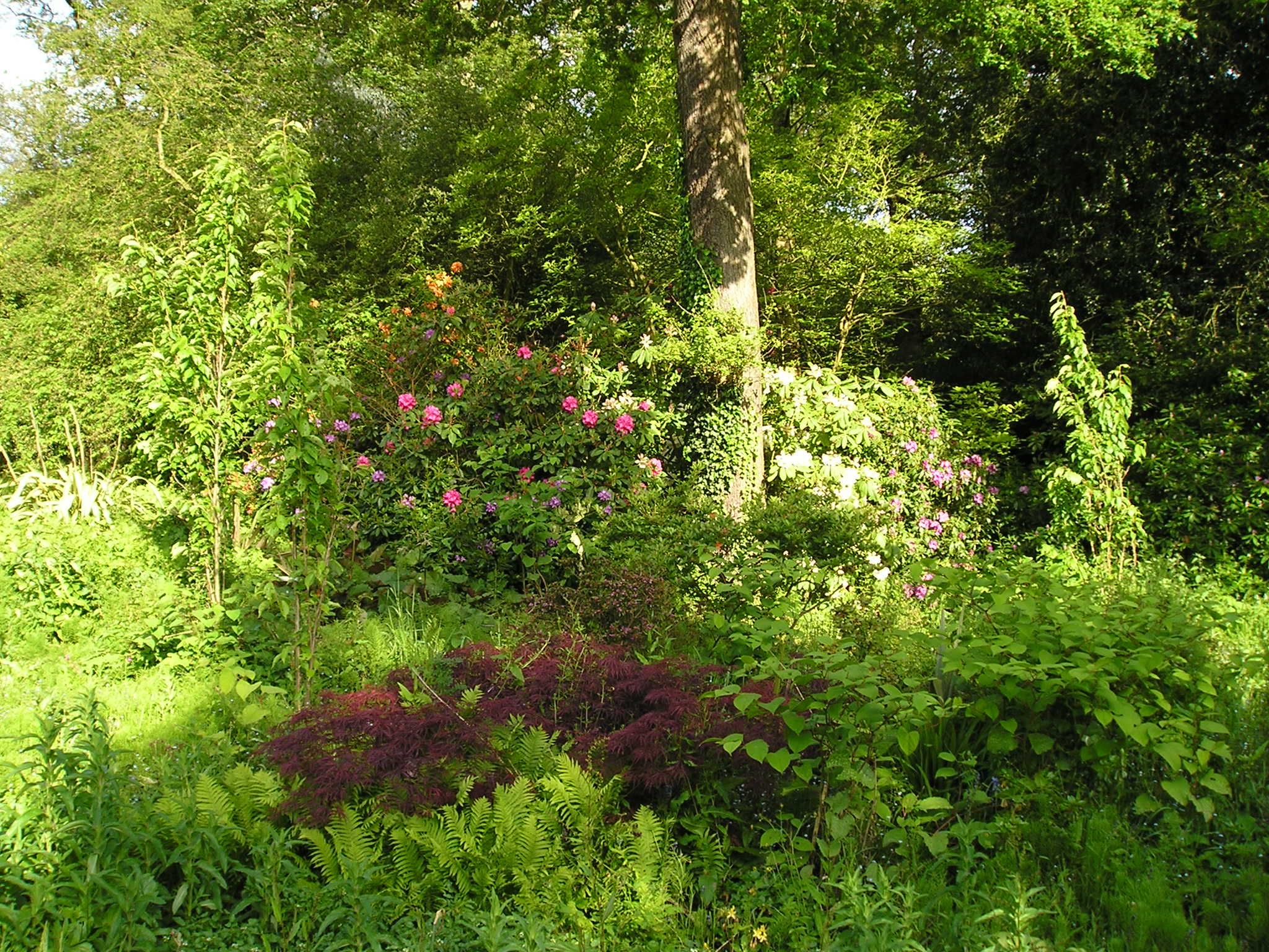
Biodiversity in Cannizaro Park, south-west London
It is no shortcoming of this list that it could apply to almost any large city. However, it is one-sided in focussing on benefits and ignoring costs. Consideration might have been given in the physical category to effects on hay-fever sufferers, and in the social category to the risks of crime in green space (some may recall the Rachel Nickell murder on Wimbledon Common in 1992 (11)). In the economic category, higher property values benefit homeowners, but disadvantage those seeking to become homeowners. Then there is the most important cost of all: the opportunity cost of the land – its value in its most valuable alternative use.
Not all these benefits apply to all types of green space. Broadly, the physical and social benefits only apply to publicly accessible green space. The environmental benefits apply to all green space, although the extent to which they apply to particular sites depends on the local geography, type of vegetative cover, and other variables.
Finally, although carbon capture by green space in London is certainly a benefit, it is just a very small contribution to carbon capture by vegetation worldwide, helping to mitigate the rise in the global level of atmospheric CO2 and so to moderate climate change. It does not provide a benefit specific to London.
Notes and References
1. City of London Corporation & BOP Consulting (2013) Green Spaces: the Benefits for London http://www.cityoflondon.gov.uk/business/economic-research-and-information/research-publications/Pages/Green-Spaces-.aspx
2. City of London Corporation, Press Release 9 July 2013 http://www.cityoflondon.gov.uk/about-the-city/who-we-are/media-centre/news-releases/2013/Pages/london-is-europe%E2%80%99s-greenest-major-city0710-5217.aspx
3. 1 acre = 4,840 square yards = 4,047 square metres = 0.4047 hectares. So 35,000 acres = c 14,200 hectares. Greater London’s area is c. 1,600 square kilometres = 160,000 hectares. Hence 35,000 acres represents 14,200 / 160,000 = c 9% of the total area.
4. See Table 2 on p 2 of 1 above. Only 4 of the cities listed are in Europe.
5. Greater London Authority Generalised Land Use Database 2005 http://data.london.gov.uk/datafiles/environment/land-use-glud-borough.xls (Although originally a UK government initiative, this data appears to be no longer available on UK government websites.)
6. Centre for Research on Environment Society and Health (CRESH) http://cresh.org.uk/cresh-themes/green-spaces-and-health/ward-level-green-space-estimates/
7. State Statistical Institute Berlin-Brandenburg Berlin in Figures 2010 p 2 https://www.statistik-berlin-brandenburg.de/produkte/faltblatt_brochure/berlin_in_Zahlen_engl.pdf
8. London: 38% of total area 1,600 square kilometres = 608 square kilometres = 608,000,000 square metres, divided by population 7,825,000 = 78 square metres per person. Berlin: 34% of total area 892 square kilometres = 303 square kilometres = 303,000,000 square metres, divided by population 3,443,000 = 88 square metres per person.
9. As 4 above.
10. 1 above, p 6 ff
- Wikipedia Murder of Rachel Nickell http://en.wikipedia.org/wiki/Murder_of_Rachel_Nickell