Economic Droplets

In a previous post I proposed, as one element in the UK’s climate change policy, a tax on the sale of beef with the aim of reducing beef production and so reducing methane emissions from cattle.  Here I consider the issue in more depth, in Q & A format.

Most discussions of climate change focus on the role of carbon dioxide emissions from fossil fuels.  What is the issue with methane?

Methane is a greenhouse gas and so contributes to climate change.  The warming potential of different greenhouse gases is often compared in terms of CO₂ equivalent, normally defined as GWP100 which compares the warming potential of a tonne of the gas with that of a tonne of carbon dioxide over a period of 100 years.  On this measure methane has a value of 28, implying that its warming potential is very high.  Of the UK’s total greenhouse gas emissions in 2023, weighted according to GWP100, carbon dioxide accounted for 79%, methane for 15% and other gases for 6% (1).

Doesn’t methane in the atmosphere gradually decay, unlike carbon dioxide?

Yes, comparison in terms of GWP100 does not give the full picture.  Methane is a short-lived greenhouse gas, its average lifetime in the atmosphere being about 12 years (2).  So although its warming potential in terms of GWP100 is 28, most of that warming occurs early in the 100 years from emission of a unit of methane, and only a little towards the end (whereas warming due to a unit of carbon dioxide occurs almost uniformly over time). 

So the methane emitted at any time is simply replacing the decaying of the methane emitted in previous years, not adding to the total methane in the atmosphere?

This is so if methane emissions are at a steady rate over time.  In fact, methane emissions in the UK have been gradually falling over time (3), implying that current emissions are somewhat less than would replace the decay of previous years’ emissions.  It can be inferred that total atmospheric methane attributable to the UK is gradually falling.

That sounds like good news.  Doesn’t it mean that the UK is already achieving its net zero target so far as methane is concerned?  Shouldn’t we therefore leave well alone?

It is good that atmospheric methane decays, rather than accumulating like carbon dioxide.  It is also good that the UK’s methane emissions are falling.  If net zero is taken to include atmospheric decay as well as emissions and withdrawals, then it could be said that we are achieving net zero in respect of methane.  Nevertheless, over the period in which a unit of methane is in the atmosphere, it contributes to the overall greenhouse effect during that period.  So long as the combined effect of carbon dioxide, methane and other greenhouse gases is producing global warming, a reduction in emissions of any of those gases would help to mitigate the warming. The fact that the methane is just replacing methane from previous years does not alter this.

Another way of thinking about this is to compare possible paths to the net zero target for total greenhouse gases.  Because methane decays, we could get very close to net zero by reducing emissions of carbon dioxide and other greenhouse gases to nil, while keeping methane emissions at their current level.  But if we also reduce methane emissions, we can get to net zero by a different path, one with less warming during the period before net zero is reached.  It has been shown that this could make the difference between achieving and failing to achieve the Paris Agreement target of holding the increase in average global temperature to no more than 2°C (4). 

What happens when methane decays?  Are there any issues with the decay products?

The main decay process is oxidation of methane to form carbon dioxide and water vapour.  Although carbon dioxide is a greenhouse gas, the significance of its formation from methane should not be over-stated since, as explained above, its warming potential is much less than that of an equivalent unit of methane.  This is, however, a small additional reason why it is desirable to reduce methane emissions.  Water vapour is also a greenhouse gas, but since it readily leaves the atmosphere as precipitation and enters via evaporation it does not contribute to climate change in the same way as other such gases.

Do any international agreements explicitly require action to reduce methane emissions?

Not exactly. The Global Methane Pledge, launched in 2021 at COP 26 and now with 160 participating countries, consists in an agreement to take voluntary actions to contribute to a collective effort to reduce global methane emissions by 30% from 2020 levels by 2030 (5).  Thus it does not require each country to reduce its methane emissions by 30%.  In 2023, a small number of the countries, of which the UK is one, agreed to act as “GMP Champions” with the roles of advocating for methane action and accelerating implementation of the Pledge (6).  The UK’s methane emissions in 2023 (the latest available) were some 5% below the 2020 level (7), so significant further reductions would be needed to achieve the 30% target by 2030.  It is fair to add however that the UK’s 2020 level was already no less than 60% below its 1990 level.

Why should there be particular concern about methane emissions from cattle and sheep?

Of the UK’s methane emissions in 2023, 48% were associated with livestock.  The other main sources were waste disposal via landfill (25%), land use and land use changes, including near-natural peatland (10%) and leakage in gas distribution (5%) (8).  Emissions from landfill have already been greatly reduced since 1990, largely via the effect of the Landfill Tax introduced in 1996, and those from gas leakage are also greatly reduced (9).  Emissions associated with livestock, however, are little lower than in 1990.  They are an example of what economists term a negative production externality because farms do not bear the cost of the harm caused by the emissions, there being no equivalent of the Landfill Tax in respect of livestock.

The break-down of the 48% livestock percentage is cattle (37%), sheep (8%), and all others including pigs and poultry less than 3% (10).  The main reason why methane emissions from cattle and sheep are relatively high is that they are ruminants, producing methane via a digestive process known as enteric fermentation (11).  Pigs and poultry are not ruminants and have different types of digestive systems which produce far less methane.  Methane emissions are also generated in the management of manure from all kinds of livestock, but these are small relative to those from enteric fermentation in ruminants (12). 

Can the cost of the harm caused by methane emissions be quantified?

It can be estimated very approximately.  Readers may have heard of the ‘social cost of carbon’ – the cost of the damage done by each additional tonne of carbon dioxide emissions – and may be aware that estimates of its magnitude depend greatly on the assumptions of the underlying models.  Estimates have also been made of the social cost of methane (SCM), and these also depend on the assumptions made.  Azar et al (2023), using a refined version of the DICE model developed by Nordhaus,  obtained a base estimate of US$ 4,000 per tonne but within a range, depending on model assumptions, of US$ 880 – 8,100 per tonne (13).  This is equivalent in £ per kilogram of CO₂ equivalent to 12p within a range of 2.5 – 23p (14). 

Aren’t  the methane emissions from some other countries, just like the carbon emissions, much higher than those from the UK?

Yes. On the basis of the above base estimate the cost of the harm done by annual anthropogenic methane emissions globally is very approximately £1.2 trillion of which those from the UK contribute about £7 billion, about 0.6% (15).  No action by the UK alone is going to solve the problem of climate change.  But equally, it is wrong to suggest that the UK has no responsibility for climate change mitigation.  A unit of methane emissions from the UK does exactly as much harm as a unit from any other country.  The UK’s main responsibility in respect of climate change mitigation is to mitigate the harm done by its emissions, and £7 billion of harm is certainly not a trivial quantity.

How are methane emissions from cattle and sheep measured, and how reliable are the measurements?

This is a complex question.  The methodology underlying the government’s aggregate emissions figures for emissions from enteric fermentation for the whole of the UK may be found in the UK’s 2024 submission to the UN Framework Convention on Climate Change (16).  This is not an easy document to understand, but those with some understanding of quantitative research methods will see that the figures are statistical estimates, not measurements as the term is normally understood, that the estimates rely on formulae relating emissions to dietary intake; and that there are numerous other complications which may be possible sources of error.  To say this is not a criticism – the methodology may well be the best available given current technology, and having approximate figures is certainly better than having no figures at all.  I should also add that, although the figures are estimates, I can see no grounds for thinking that they are biased estimates: they are as likely to be under-estimates as over-estimates.

What about measurement at the level of individual animals or farms?  That is important for several reasons.  Any aggregate estimates must ultimately be supported by at least a sample of measurements at individual level.  The same applies to any research on the effectiveness in reducing emissions of methods such as changes in diet.  Reliable figures at farm level are also an essential requirement for any policy designed to incentivise farms to reduce their emissions.  Unfortunately, the available methods all have limitations.  Some focus on individual animals and require that an animal be confined in a chamber, or have an insertion into its stomach and/or a tube connected to its nose, or require use of a hand-held laser methane detector (17).  Some attempt to measure emissions in a whole building or field, but these can hardly be expected to yield accurate results given the dispersive effects on methane of ventilation and wind (18).  There are also lab-based methods which simulate in vitro the fermentation process occurring in the stomachs of ruminants so as to determine the relationship between animal feed and methane emissions (19), but these, by their very nature, are ways of estimating, not measuring, emissions from actual animals. 

A further complication arises in analysing the emissions from cattle between production of beef and production of milk.  Cows raised primarily for their milk must give birth to calves, some of which are not required to maintain the numbers of adult dairy cows and are slaughtered to produce veal, which for statistical purposes is generally included within beef production.  Thus part of the emissions from dairy herds should be attributed to beef rather than to milk, but there is no clearly correct method to determine what that part should be. 

For these reasons, all the figures in what follows should be understood as very approximate.

How much methane is emitted in the production of a unit of meat or milk?

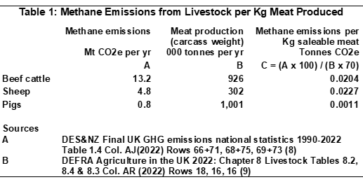
The following figures measure methane in terms of carbon dioxide equivalent (CO₂e)  calculated on the GWP100 basis.  They are derived from the aggregate emissions figures described above together with aggregate UK production data.  Production in the UK of one kilogram of beef or lamb is associated with emission of about 20 kilograms CO₂e of methane, while production of one kilogram of pork is associated with emission of just 1 kilogram CO₂e of methane (20).  The available data does not support calculation of a figure for chicken but, because chickens are not ruminants, the figure is likely to be similar to or even lower than that for pork. 

Production of 1 kilogram of cow’s milk (which is very close to the weight of 1 litre) is associated with emission of about 0.6 kilograms CO₂e of methane (21).  Although dairy cattle are ruminants, just like beef cattle, the very large quantity of milk a cow can produce over its lifetime (about 30,000 kilograms (22)) means that methane emissions per kilogram of milk are low. 

Those figures are very different from some I have seen elsewhere?  Why is that?

The above figures are calculated from UK data.  Some websites quote figures which are global averages.  For example the website Our World in Data (23) includes a graphic based on figures from a paper by Poore & Nemecek (2018) which are global averages.  One reason why UK figures tend to be lower than global averages is that most livestock grazing in the UK is on land that has been grazed for many years, so that any deforestation needed to convert the land to pasture took place long ago.  In some countries, notably Brazil which is one of the largest producers of beef, much grazing is on recently deforested land, and deforestation can lead to methane emissions through its effects on soil and soil microbes (24).

Different approaches to allocating the emissions from dairy herds between beef and milk may also contribute to these differences.

Isn’t it more useful to compare nutritionally equivalent quantities?

In principle yes, although meat and milk contain many different nutrients, so the concept of nutritional equivalence is not straightforward.  They are valued primarily as sources of protein, so it is probably most useful to compare quantities containing equivalent amounts of protein.  Even then, however, some cuts of beef, for example, contain less protein (and more fat) than others, so precise numbers should not be expected.  As a first approximation, the protein contents of the different meats are fairly similar, so the above comparisons between beef and lamb on the one hand and pork and chicken on the other do give a valid picture.

Milk, however, contains only about one seventh as much protein as meat per kilogram (25).  To provide protein equivalent to that in 1 kilogram of meat would require about 8 litres of milk, production of which would be associated with emission of about 5 kilograms CO₂e of methane (26).  In that sense, the methane associated with production of milk is much more than that associated with production of pork or chicken, but very much less than that associated with production of beef or lamb.

What about other protein-rich foods that people might choose to substitute for beef and lamb?

The Poore & Nemecek paper quotes figures for the greenhouse gas emissions from production of a variety of foods per 100 grams of protein content.  Its mean figures for all its listed alternatives to meat, which include fish (farmed), crustaceans (farmed), eggs, cheese, tofu and nuts, are all much lower than those for beef from beef cattle and lower than those for lamb and mutton (27).  In comparison with its figure for beef from the dairy herd, the figures are lower for all the listed alternatives except crustaceans (farmed) for which the figure is very slightly higher (28).  All these figures are global averages: however high proportions of fish, crustaceans, tofu and nuts consumed in the UK are imported (or in the case of tofu produced from imported soya beans), so figures for UK production would not be especially relevant.

Don’t livestock have other environmental impacts, some of which are highly beneficial?  Doesn’t meat and milk production generate positive as well as negative externalities?

Yes.  On the harmful side, management of livestock manure produces emissions of nitrous oxide, another greenhouse gas, although the amount, in terms of CO₂e, is small relative to the methane emissions from cattle and sheep (29).

However, livestock provide several kinds of environmental benefits. So far as greenhouse gases are concerned, pasture permanently grazed by livestock sequesters carbon dioxide.  Data is available for the annual amount sequestered by all grassland (whether grazed or not): in terms of CO₂e, this is about one fifth of the methane emissions from livestock (30).  Permanent grazing also preserves certain ecosystems and so supports certain wildlife, with both use value (to recreationists who enjoy the countryside and/or observing wildlife) and non-use value (arising simply from the existence of species).  These are positive externalities because the various benefits are not solely to the farmers themselves. 

In order to assess the environmental benefits of livestock grazing, shouldn’t one also consider how the land might be used if it were not grazed?

Yes. While grassland grazed by cattle or sheep is a traditional rural landscape, as it now exists it is far from being a natural landscape, untouched by any kind of human intervention.  A truly natural landscape might have been grazed by wild ancestors of cattle or sheep, but those animals would not have been protected from disease or predators, the grass on which they grazed would not have been improved by artificial fertilisation or seeding, and the animals would not have been milked or slaughtered for human consumption.  Converting land from livestock grazing to some other use, then, is not destroying nature: it is converting it from one at least partly human-determined use to another.

It is helpful to divide alternative uses into three categories.  Firstly, there are those which would provide most but not all of the same environmental benefits as grazed land.  The obvious example is land converted to ungrazed grassland, which would still provide most of the same ecosystem services such as soil carbon sequestration and nutrient cycling, would still provide a habitat for some of the same wildlife, and could be open to recreational visitors to the same extent as before.  The difference would be that it would not support exactly the same wildlife: without grazing it would not support species dependent on livestock such as dung beetles, and as a consequence would not support bird species that feed on them. 

Secondly, there are alternative uses which would provide alternative environmental benefits which might be of equivalent or even greater value.  That would include conversion to woodland, either through planned tree planting, or by natural progression from unmanaged grassland via scrubland.  Although this would take many years, the quantity of carbon that the trees might sequester suggests that the total environmental benefit could be greater than that from grazed land, albeit with a very different composition.  This category could also include  conversion for uses providing indirect environmental benefits including pig and poultry farming and solar farms, the benefits being facilitation of substitutes for meat from ruminants and for energy from fossil fuels.

Thirdly, there are alternative uses which would almost certainly lead to a loss of environmental benefits, including residential or industrial development. 

If one wanted a maximum estimate of the loss of environmental value from discontinuing grazing, one might focus on the case of conversion to urban development.  To minimise the estimated loss, one might focus on conversion to woodland.  Common sense suggests however that there would be various alternative uses, and that at most some but not all of the net environmental value that might be identified with grazing would be lost.  If a large proportion of any lost grazing land were converted to woodland, then the net change in environmental value might well be positive.

How can the UK achieve a reasonable balance between reducing methane emissions from cattle and sheep, preserving environmental benefits, and continuing to produce meat and milk for consumers?

Three broad approaches are possible, focusing respectively on reducing emissions per cow or sheep, reducing livestock numbers per unit of output of beef, lamb or milk, and reducing output of those products.  The first approach, to the extent that it is feasible, is straightforward, implying no change in livestock numbers, areas grazed or meat and milk output.

The other two approaches are more complicated.  Both require a reduction in numbers of cattle and sheep.  The second approach aims to improve productivity, so that the same output is achieved from fewer cattle and sheep and therefore with less emissions.  The third approach accepts a reduction in output of beef, lamb and milk (which might be offset by an increase in output of other protein-rich foods) as a means of reducing emissions.  In order to preserve most of the environmental benefits, both these methods also require that the locations converted from grazing to other land uses, and the choice of their new land uses, should be such as to limit the loss of environmental benefits.

The second and third approaches above seem to assume that, of the overall environmental benefit from grazing, much more is provided by some areas than by others.  Is that really so?

It is, for two kinds of reasons. 

The more obvious reason is that some locations have special characteristics that make their use or non-use values especially large.  For recreational use these include areas of outstanding natural beauty and locations which, though perhaps not outstandingly attractive, receive many visitors because they are within easy travelling distance of large centres of population.  For non-use values, they include locations with unique or rare ecosystems and habitats of rare species.

A more technical but still important reason is that the distinction between total and marginal values, widely used in economics, is just as applicable to environmental values.  Suppose there are ten fairly similar areas of grazed land in a region, none with special characteristics such as described above, all visited by small numbers of recreationists.  Now suppose one of those ten areas is converted to some other land use so that it becomes either unattractive or inaccessible.  The loss of use value will normally be quite small, not just because the number of recreationists who visited the area was quite small, but also because some, perhaps most, of those recreationists will instead choose to visit one or more of the remaining nine areas, gaining similar enjoyment from so doing.  If however nine of the ten areas are converted to such alternative use, the loss of value will be much more and, crucially, much more than nine times as much.  For if only one of the ten areas remains, two effects are likely to be significant.  A considerable proportion of the recreationists who used to visit any of the other nine areas will find the one remaining area less convenient to access due to distance.  Nevertheless, another considerable proportion will instead visit the remaining site, which as a consequence will change in character, receiving many more visitors and offering less of the unspoilt rural ambience many visitors value.  Should the tenth area also be converted, then the loss of value will clearly be even more, with similar experiences available to the former visitors only at the cost and effort of travelling right outside the region.  It is only then that the total value of the ten areas is lost.

Somewhat similar considerations apply if ten areas in a region form a unique ecosystem or habitat of a rare species.  Loss of one or two areas will probably not have severe ecological consequences.  But as more areas are converted to alternative uses the consequences may become much more severe.  The converted areas may become barriers hampering movement between the remaining areas to find food or mates, or sources of invasive species changing the character of the ecosystem.  Species populations may become too small to be viable. 

Emphasising the total benefits of some feature of the countryside when the consequence of a possible change would only be a loss of marginal benefits is an easy route to poor policy.

What methods are available to reduce methane emissions per cow or per sheep?

Since most of the emissions are generated in digestion, appropriate changes in livestock diets can reduce emissions.  One method is to improve the quality of pasture in diets.  Pasture which is more digestible and has higher nutrient quality can reduce enteric fermentation (31).  Improvements may be achieved by pasture management (periodic fertilisation, re-seeding, etc) and also (where livestock is only seasonally fed on pasture) by grazing at the time of year when quality is highest.  Another method is to increase the use of concentrates (eg grains, maize and fats) and rely less on pasture and hay.  Reduced intake of high-cellulose food such as grass can reduce enteric fermentation (32). However, any such reduction in emissions may be partly offset by increased emissions in production of the concentrates. Also, grass-fed beef is perceived by many consumers as better-tasting, healthier and more natural. 

A quite different method which has been the subject of considerable research in recent years is the use of feed additives designed or found to reduce emissions.  Many have been tried; the following are among those which have gained most interest.

3-nitrooxypropanol is a synthetic chemical which interferes with the generation of methane in animal stomachs.  Emissions reductions have been estimated at 39% for dairy cattle and 17% for beef cattle (33).  It is marketed as Bovaer by dsm-firmenich, a Switzerland-based international company, and has been approved for use in the UK by the Food Standards Agency (FSA) (34) (so far as I am aware it is the only methane-suppressing additive which has received such approval).

Asparagopsis taxiformis is a species of red seaweed containing bromoform which inhibits the generation of methane in animal stomachs.  Some studies have found emissions reductions of more than 50%,  although some found reductions did not persist and milk yield was reduced (35).  It is marketed by Future Feed, an Australian company.

Various essential oils have been found to reduce methane emissions, although reductions are often small (c 10%) (36).  One combination is marketed as Agolin Ruminant by Agolin, part of the US-based Alltech group. 

It has been found that emissions from different breeds of dairy cattle can differ by c 20% with no difference in output (37).  This suggests that emissions might be reduced by appropriate choice of breeds and perhaps, in the long term, by selective breeding.  However, many other factors need to be considered in choice of breeds, eg suitability for local climate and resilience to disease.

Aren’t concentrates already a significant part of the diet of many UK cattle and sheep?

Yes, most cattle and sheep in the UK already have diets which, though largely consisting of pasture and forage, also include significant quantities of concentrates. Admittedly, that might not be the impression one gains at the meat shelves of supermarkets, where it is common to see packs of beef prominently labelled ‘grass fed’.  However, such labelling should not be taken to imply that the beef is from cattle that are 100% grass fed.  One supplier, for example, includes on its packs of beef the words ‘grass fed’ but also, in smaller lettering, ‘70% guaranteed grass-based diet’ and ‘180 days grazing naturally in fields’ (38). 

An indication of the extent to which the diet of UK cattle and sheep includes concentrates is given by national consumption statistics.  UK annual consumption of concentrates for cattle is about 5 M tonnes; for sheep feed the figure is 800,000 tonnes (39).  The main raw materials used are wheat, barley, maize, oilseed rape and soya (40).  Given that the UK population of cattle is about 9 million (41), this means that cows consume on average at least 500 kilograms of concentrates per year or well over 1 kilogram per day.  So, while a small proportion of UK cattle are reared on a diet consisting almost entirely of pasture and forage, UK cattle farming as a whole is not starting from that position.  Similar considerations apply to sheep.

What methods are available to reduce emissions by improving productivity?

Some of the methds outlined above can also in some circumstances raise output per animal.  This applies to improved pasture quality (42) and to the additive Agolin Ruminant (43).

Productivity can also be improved via the use of growth hormones, which can improve the efficiency of conversion of feed, enabling animals to be fattened in less time, a shorter lifespan implying, other things being equal, less emissions per unit of meat output.  However, there are concerns about the effects of growth hormones on animal welfare and human health.  Their  use is illegal in the UK (and also in the EU, though legal in the US).

How reliable is the research on these various methods?

While much good work has been done, there are several reasons why these research findings should be treated with caution.  Firstly, claims regarding percentage reductions in emissions must depend on measurements of emissions, which as discussed above are unlikely to be highly accurate (this point applies in particular to the efficacy studies forming part of the FSA’s assessment of Bovaer).  Secondly, it is well-known that many scientific journals are reluctant to publish negative results (44): hence the literature may give a somewhat over-optimistic impression of the potential of these methods.  Thirdly, an ideal method would be effective in dairy cattle, beef cattle and sheep, but many studies relate to one type of animal only, with studies on sheep appearing to be scarce.  Fourthly, although many studies have investigated the effects of various methods on actual farms, most such studies have been on farms outside the UK.  It could be that the same methods would have somewhat different effects if used in the UK, given its climate, soils and farming practices.  Fifthly, so far as methods involving changes in diet are concerned, the potential for reducing emissions will clearly depend on the dietary starting point.  As explained above, there is already significant use of concentrates in UK livestock diets.

Further considerations apply to research on the various feed additives. While many studies consider possible adverse side-effects on milk or meat output or animal health, or other possible disadvantages such as diminishing efficacy over time, it is not clear that these have yet been studied as fully as they might, particularly in respect of possible long-term or cumulative effects.  Some studies have authors associated with commercial interests (45).  I have not seen in the literature a satisfactory explanation of how feed additives could routinely and conveniently be administered to animals grazing in fields. 

How would you sum up the position on these methods of reducing methane emissions so far as the UK is concerned?

Four broad conclusions can be drawn.

Further research on these methods is needed, including trials of different methods under actual farm conditions found in the UK. 

It seems likely that one or a combination of these methods will soon make possible a significant reduction of methane emissions per unit output from ruminants on UK farms.  However, it is not yet clear which method(s) is/are best, having regard to possible side-effects as well as effectiveness in reducing emissions.

The extent to which the possible reduction is actually realised will depend on the behaviour of farmers and consumers and on government policy.  Whether consumers will accept meat or milk from animals that have been fed methane-suppressing additives, for example, is largely untested.

Even with full acceptance by farmers and consumers, the reduction in emissions per unit output is unlikely in the foreseeable future to exceed 50%.  The remaining 50% or more  will continue to make a significant contribution to climate change unless addressed by reducing ruminant numbers and output.

What is the current position on trials of these methods in the UK?

Some trials in the UK have already taken place or are planned.  In 2022, a government call for evidence on methane-suppressing feed products asked respondents about trials on their farms or in their supply chains.  Out of just over 100 responses from farm businesses, 20% stated that they had previously trialled, were currently trialling or planned to trial such products.  Among about 80 responses from other organisations including farm suppliers and advisors, manufacturers and trade bodies, the corresponding figure was almost 50% (46).  More recently, ARLA Foods, a large farmer-owned company specialising in production of milk and milk-based products, announced that in conjunction with supermarket chains Morrisons, Tesco and Aldi it would be conducting a large-scale trial of the use of Bovaer (47).   

One might argue that, since research and trials are taking place anyway, there is no need for policy intervention.  However, it is far from clear that they are addressing the full range of questions that need to be addressed.  The ARLA trial, rather than comparing different feed additives in respect of effectiveness and other characteristics, relates specifically to Bovaer.  It would be unfortunate, and potentially add to the cost of reducing emissions, if a situation were allowed to develop in which one company had an effective monopoly of supply in the UK of methane-suppressing additives. 

What should be done to ensure the undertaking of appropriate further research and trials?

I propose as follows:

Proposal A: The government should offer financial support, via the appropriate Research Councils, for research and trials to improve knowledge of the effectiveness and other characteristics under conditions on UK farms of different methods of reducing methane emissions from ruminants.  This should include comparisons of different feed additives.  It should also include research aiming to develop improved and more accurate methods of measuring methane emissions from farms.  

This proposal does not necessarily require additional government expenditure.  It may be that it can be achieved simply by a review of priorities on the part of the relevant Research Councils. 

The proposed involvement of Research Councils is not merely a means of channelling funding at arm’s length from government.  It also ensures that research is undertaken within a framework promoting high standards of integrity upholding the values of honesty, rigour, transparency and openness (48)(49), the latter ensuring that findings are available to interested parties and facilitating attempts to establish the reproducibility or otherwise of research findings and to determine to what extent such findings remain valid under different conditions.  These points are not minor details: they are an essential foundation for building trust and countering misinformation among consumers, without which even safe and effective feed additives could fail to win acceptance. 

What advantages are there in the third approach for reducing emissions, that is, by reducing output of beef, lamb and milk?  Surely this should be a last resort?

There are several advantages.  Firstly, it is a method which quite definitely works.  No further reearch is needed to confirm that a reduction in cattle and sheep populations will result in a reduction in emissions, or to rule out the possibility of adverse side-effects to animals or consumers.  Secondly, unlike the other two methods, it has the potential to reduce emissions from cattle and sheep by any desired percentage, subject of course to accepting the consequences for livestock populations and output.  Thirdly, the preferences of some consumers – and I emphasize the word ‘some’ – are such that they would require little incentive to replace beef and lamb in their diets with meats from non-ruminants such as pork and chicken or with other protein sources.

Greenhouse gas emissions are just part of the ecological footprint of food production.  Is it really better environmentally to consume more of other protein sources and less beef and lamb when the full ecological footprint of their production is considered?

In most cases it appears to be better, simply because the advantage of most other protein sources in lower greenhouse gas emissions and lower land use is so great as unlikely to be outweighed by other environmental considerations.  Relevant data may be found in the Poore & Nemecek paper which also includes figures for acidification, eutrophication and freshwater withdrawals (50).  However there could be exceptions. The most likely appear to be where water-intensive methods are used to produce nuts or farmed fish or crustaceans in regions subject to water scarcity. 

It is impossible to give a conclusive answer to the question because there can be reasonable disagreement as to what is better environmentally.  Most fundamentally, should we emphasize the preservation of nature or the sustainable meeting of human needs?  And where there are trade-offs between different environmental features, land use and water consumption say, how should we weight the features?  One way to formulate my argument above is to say that consuming more of other protein sources and less beef and lamb is better in most cases unless greenhouse gas emissions and land use are assigned a very low weighting relative to other environmental features.

There is also the contentious issue of the relative weighting of environmental consequences in the UK and those elsewhere in the world. My view, in simple terms, starts from the observation that a rough distinction can be made between creating environmental benefits and avoiding environmental harm.  I then assert that it is entirely reasonable to prioritize one’s own country in creating benefits: just because a government funds say the creation of a national park in its own country, it is not under any sort of obligation to fund similar projects in other countries.  However, the same does not apply to avoidance of harm, with mitigation of greenhouse gas emissions being a clear example.  It would be quite wrong, in my view, to give a low weighting to mitigation of such emissions on the grounds that most of the resulting harm occurs outside the UK and especially in tropical and sub-tropical regions. 

If there could be exceptions, that is, other protein sources which are not environmentally better than beef and lamb, doesn’t that undermine any case for reducing output of beef and lamb?

No, the solution would be to adopt, in addition to any policies regarding beef and lamb, policies to address the environmental consequences of production of those particular other protein sources.  Although the possibility of exceptions can be admitted, this does not alter the fact that, on any reasonable criteria, there are a range of protein sources which are environmentally better than beef and lamb. 

Wouldn’t some consumers be willing to make changes in their diets even without any incentive, if only there were more  awareness of the climate implications of beef and lamb production?

This is quite possible.  It seems a reasonable supposition that there are people and households who: a) recognise that climate change is a serious problem; b) would be willing to change their behaviour so as to reduce their ‘greenhouse gas footprint’ if the cost / disadvantage to them were not too great; but c) are unaware that production of beef and lamb, but not of other protein sources, are major sources of methane, a greenhouse gas.  Even if only a small proportion of consumers meet all three conditions, measures to increase awareness could be a low-cost means of achieving some reduction in emissions.  Hence my next proposal:

Proposal B:  The government should take suitable steps to promote awareness of the link between beef and lamb production and climate change, and of the climate benefits of switching to other protein sources.  Such steps might include mention in dietary guidance such as the Eatwell Guide, requirements on food labelling, and mention in ministerial speeches and communications. 

As well as prompting some consumers to change their diets once aware of the link, such steps would also help to prepare the public for other policy interventions designed to reduce methane emissions from cattle and sheep.

Whatever the case for reducing output of beef and lamb, shouldn’t milk be treated differently?

Yes, for four reasons.  One is that, as explained above, methane emissions from production of milk per nutritionally equivalent unit are much lower than those from production of beef and lamb.  Another is that, whereas different types of meat are generally recognised as close substitutes for each other, there is no generally recognised substitute for cow’s milk.  Alternatives such as soya milk and oat milk have gained a degree of acceptance with some consumers, but demand is still a tiny fraction of that for cow’s milk.  In 2023, UK sales of all plant milks were 242 million litres (51), while those of cow’s milk were almost 6 billion litres, about twenty-four times larger (52). 

The third reason relates to political feasibility.  A proposal to reduce production and consumption of beef and lamb, for which substitutes are available, may be considered a sensible pushing of the boundaries of politically acceptability.  Many people are already aware of advice, independent of climate considerations, that reducing consumption of red meat would benefit their health (53).  I do not think the same can be said for production and consumption of milk, which is widely perceived as playing a vital role in the nutrition of growing children.  Although the parallel is far from perfect, I recall the outrage expressed by many when, in 1971, the then government decided to end the practice of providing free milk to children in schools (54). 

The fourth reason arises from the need for balance between reducing methane emissions and preserving the environmental benefits of livestock grazing.  It is much easier to preserve most of those environmental benefits if any policy intervention to reduce such grazing is limited to beef cattle and sheep, so that large areas of pasture grazed by dairy cattle will certainly be unaffected.

So far as the other two approaches to reducing emissions are concerned, that is, reducing emissions per cow or sheep, and reducing livestock numbers per unit of output, these are just as suitable for milk as for beef and lamb.  The above reasons amount only to a case against reducing emissions by reducing milk output.

If the government adopts an approach of laissez-faire in respect of methane emissions by beef cattle and sheep, other than via research and trials and promotion of awareness, will emissions fall significantly from current levels?

This seems unlikely.  Greater awareness on the part of consumers may lead to some reductions, and some climate-conscious farmers may, even at some cost to themselves, take steps to reduce their emissions.  There may also be a gradual fall in consumption of all red meats prompted by health considerations and greater availability of plant-based protein sources.  However, there are many other issues competing for consumers’ attention, and many consumers will not perceive climate change mitigation as an issue for them.  Many farmers, often operating with narrow profit margins, will be reluctant to incur extra costs to reduce their emissions.

Thus any significant reduction in emissions is likely to require government intervention.

Of the various methods of reducing methane emissions by beef cattle and sheep, which show the most promise as bases for effective government intervention?

The most promising for early implementation is reducing output of beef and lamb. Its advantages have been explained above.  What policies should be adopted to bring about such a reduction will be considered below.

Methane-suppressing additives also have considerable promise, but I do not think the government should encourage their use at present, other than for purposes of research or trials. The time may well come when our level of knowledge is sufficient to justify stronger government action, but premature action would carry a number of risks. These include choice of one additive that turns out to be less effective than another, unnecessary extra costs in the event that one company is allowed to become the sole source of permitted additives, adverse effects on animal productivity, and harm to animal or human health.  Of course it is possible that none of these consequences will ensue, and it is also true that it may be impossible ever to achieve full certainty that there is no risk of any kind.  As in many areas of policy formulation, a key element is judgment about degrees of risk, and my judgment is that the degree of risk relating to methane-suppressing feed additives is, as at 2025, not small enough to justify incentivising or mandating their use.

I would not normally present a recommendation to take no action as a formal proposal, but in this case it is appropriate to do so since the UK’s Climate Change Committee has recommended that the government “mandate the addition of methane-suppressing feed additives to feed products for UK beef and dairy systems” (55):

Proposal C: The government should not, at present, mandate the use of methane-suppressing additives for cattle and sheep.  It should, however, keep under review the progress of research on and trials of such additives with a view to mandating their use if and when there is sufficiently strong evidence that they are effective, economic and safe both for animals and for human consumers of meat and milk when used on a long-term basis.

A case might also be made that the government should encourage the inclusion of concentrates in cattle and sheep diets as a method of reducing emissions.  However, the  practical question for most farmers is not whether they should be encouraged to include concentrates in the diets of their ruminant livestock but whether they should be encouraged to include more than, as explained above, they do already.  It is not clear that an increased intake of concentrates always reduces methane emissions.  One study, on a group of dairy cows in Chile, found that an increase in concentrates actually increased methane emissions (56). Comparison of studies in various circumstances suggests that substitution of concentrates for pasture in diets is most effective in reducing methane emissions where the pasture is of poor quality and less digestible (57), whereas much of the UK, with its normal year-round rainfall and rarity of extreme temperatures, is an excellent environment for growing good quality pasture.  In my view, the case for intervention to incentivise or mandate greater use of concentrates in the diets of ruminants does not currently meet the fairly high bar that such a case should meet, although with further research it is possible that it may do at some future date. 

Rather than choose among these bases, wouldn’t it be simpler and better just to impose on farms a tax per tonne of methane emissions?

This would in some ways be an ideal policy for reducing emissions.  It would incentivise farmers to reduce their emissions while leaving them free to determine the most cost-effective method and, equally importantly, not requiring the government to determine the best method, for which it probably lacks the necessary knowledge. 

Unfortunately, this is not a practicable policy because, as explained above, we do not currently have sufficiently reliable methods of measuring methane emissions at farm level.  Any attempt to impose such a policy would almost certainly be subject to numerous legal challenges from farms maintaining that their emissions had not been accurately measured for tax purposes.

A relevant precedent is the very successful Landfill Tax, which is based not on measured emissions from landfill, but on the weight of waste material sent to landfill (58).

What is the most suitable target for a policy to reduce output of beef and lamb?

The language of policy analysis distinguishes between objectives, targets and instruments.  For example, discouraging smoking so as to improve health is an objective, the retail sale of cigarettes is a target, and a tax on retail sales is an instrument.

Beef cattle and sheep stand at the start of supply chains driven by consumer demand for beef and lamb, with steps in the chains including not only the raising of livestock on farms but also the work of slaughterhouses, butchers, packagers, wholesalers and retail outlets. In some cases, the chains will also include processors, such as sausage and pie manufacturers. In principle, action to reduce animal numbers could be targeted at any point in those chains, since a reduction in demand at any point would impact back through the chains to farmers.  The possible targets therefore need to be assessed in terms of effectiveness, cost and side-effects, and the best selected.

Since the UK both imports and exports beef and lamb, a key consideration is to avoid two possible unsatisfactory consequences.  One would be if a reduction in UK output of beef and lamb were offset by increased imports, so that the reduction in UK emissions would be more or less offset by increased emissions elsewhere.  The other would be if UK farmers were  disadvantaged in competition with those in other countries which may not be adopting equivalent policies.  Primarily for these reasons, the most suitable target is the retail sale of beef and lamb, with domestically-produced and imported meat treated in exactly the same way. 

Admittedly the targeting of retail sales is not without disadvantages.  Depending on the instrument(s) adopted, it is likely to involve administrative costs for retailers.  There is also the issue of avoiding loopholes where meat is sold other than via a conventional retailer, for example direct from farm to consumer.  The argument here is that, weighing the pros and cons, retail sale is a better target than any other.

What is the most suitable instrument to target the retail sale of beef and lamb?

Mention has already been made, in Proposal B, of the possibility of requiring food labelling to promote awareness of the link between beef and lamb production and climate change.

Of the more forcible instruments that could plausibly be applied to retailers, the main options  are various forms of quotas and taxes.

Quotas could be related to weight of beef sold.  To be effective in reducing emissions, the overall quota would need to be set at less than the weight of beef which would have been sold in a free market.  This restriction of supply would tend to raise the price of beef, creating extra profit which, depending on various elasticities, would be shared in some manner between producers, retailers and others in the supply chain.  The main problem would be that it would fall to the government or its agency to allocate quotas, within the overall total, to particular retailers.  That could be done in various ways, including geographically by population, pro rata to previous sales, by auction (which would reduce profit and raise revenue for the government), and even making quotas tradeable. However the quotas were determined, this is in my view over-complicated, carries a risk of shortages in the event that quotas are not administered effectively or retailers misjudge the pricing of beef, and would invite unnecessary micro-management by the minister responsible and lobbying by retailers. 

My proposal, therefore, is a tax. Options include a fixed sum per unit weight, or a percentage addition to selling price.  Neither are perfect proxies for the quantity of methane emissions generated in production.  Weight is an imperfect proxy because of the different methods used to produce meat, primarily the balance between grazing and indoor housing or feedlots and, closely related, the balance of diet between grass and concentrates.  However, price is an even poorer proxy.  Different cuts of meat, even from the same animal, may command very different prices.  Beef which has been matured (aged following slaughter) to improve flavour and tenderness tends to be more expensive, but the maturing process does not add to methane emissions.  At the time of writing, prices per kilogram of beef range from about £7 for standard mince to £40 and more for premium products.

How the government should use the revenue from such a tax is outside the scope of this post.  One option, of course, is to use it to reduce some other tax: thus the introduction of a tax on beef and lamb does not necessarily imply an increase in the overall burden of taxation.  

It seems likely that the introduction of a tax, at whatever rate, would have a secondary effect of raising awareness of methane from cattle and sheep as a contributory cause of climate change.  That in itself, over and above the incentive effect of the tax, might lead some people to reduce their consumption of beef and lamb.

How effective would a tax be in reducing production of beef and lamb?

It would be fairly effective, because demand and supply of beef and of lamb are likely to be fairly elastic.  This can be explained with the aid of the following diagrams:

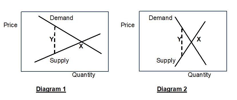
Both diagrams show demand and supply curves which, in the absence of a tax, yield an equilibrium where the demand price equals the supply price, that is, at point X where they intersect.  With a tax in place, equilibrium is where the demand price exceeds the supply price by the amount of the tax, indicated by the dashed line Y.  In both diagrams, Y is to the left of X, indicating that the tax reduces the quantity sold.  This effect will work back through the supply chain, ultimately leading to lower farm output.

The difference between the diagrams is that demand and supply are more elastic in Diagram 1, that is, the demand and supply curves slope more gently.  As a consequence Y is much further to the left of X than in Diagram 2, indicating that the reduction in quantity sold due to the tax is much more in Diagram 1. 

My contention is that the markets for beef and lamb are in the long run more like Diagram 1.  Demand for beef and lamb is likely to be fairly elastic, just because there are other kinds of meat and other sources of protein which many consumers would be willing to substitute in response to an increase in their prices.  On the supply side, substitution of other agricultural products for beef and lamb is also possible, although it takes time because of, for example, the need to convert land, purchase new livestock and equipment and develop new skills.  Thus supply of beef and lamb is likely to be inelastic in the short run but fairly elastic over a period of several years.

What is the most appropriate initial rate per kilogram of beef or lamb for a tax designed to reduce methane emissions?

As was explained above, methane emissions from livestock are an example of a negative production externality because the costs of the harm done by the emissions are not borne by farmers.  In other words, the social costs of beef and lamb production, which include the cost of the harm, exceed the private costs to farmers, the actual costs borne by farmers in the absence of policy intervention.  The standard economic approach to the use of a tax to address a negative externality is to view the tax as a means of internalizing the costs of the harm, that is, raising the private costs to farmers so as to bring them into line with the social costs.  This will shift farmers’ supply curves for beef and lamb, leading to a reduction in output of beef and lamb and therefore a reduction in methane emissions.

The imposition of a tax on retail sales rather than farmers does not invalidate this approach, although it does complicate its operation.  The tax shifts the demand curves faced by shops for beef and lamb, reducing the quantities they sell and also reducing the net-of-tax prices they receive. These changes work back through the supply chain leading to a shift in the demand curves faced by farmers for beef and lamb and, again, a reduction in output of beef and lamb.

A significant difficulty with the above is to quantify the costs of the harm done.  Using Azar et al’s estimates of the social cost of methane together with my own estimate that production of 1 kilogram of beef or lamb generates 20 kilograms CO₂ equivalent of methane, the cost of the climate damage attributable to that beef or lamb is £2.40 within a range of £0.50-4.60 (59).  That very wide range is before consideration of the approximation in the estimates underlying the 20 kilogram figure.

Furthermore, to base a tax rate on the social cost of methane does not fit well with the UK approach to climate change policy based on progressively tighter carbon budgets designed to lead to net zero by 2050.  We do not know by how much beef and lamb output and associated emissions would fall in response to any particular rate of tax.  Estimates can be made using estimates of the elasticity of demand for beef and lamb, but are unlikely to be very reliable. 

An alternative is what might be termed a trial and error approach, that is, to set a tax at an initial more or less arbitrary rate, to monitor its effect on sales and output of beef and lamb and on associated emissions, and if judged appropriate to adjust the rate in the light of experience. 

Whether an adjustment is appropriate should be judged primarily by whether the tax is delivering emissions reductions sufficient to make a worthwhile contribution to achievement of carbon budgets.  Future rates should also have regard to the extent of any emissions reductions achieved by other means such as use of methane-suppressing additives.

Given all the above considerations I propose a rate that is a round number and which can if necessary be defended as towards the lower end of the range indicated by estimates of the social cost of methane:

Proposal D: The government should announce a tax on the retail sale of beef and lamb at a rate of £1 per kilogram.  It should explain that the purpose of the tax is to reduce methane emissions so as to mitigate climate change. The rate should periodically be reviewed in the light of the effect on sales and output of beef and lamb and associated methane emissions, and on progress in reducing emissions by other means such as use of methane-suppressing additives. 

In percentage terms, such a tax would be equivalent to about 14% on standard beef mince, falling to 5% or less on premium products, with an average in the region of 10% (60).

How would such a tax affect consumers’ spending on food?

The effect on a household’s spending will depend on whether it maintains its consumption of beef and lamb or whether it to some extent substitutes other foods. Households which maintain their consumption of beef and lamb will spend somewhat more on food, other things being equal.  However, the percentage increase in their spending on beef and lamb is likely in the long run to be less than the average percentage of the tax.  As Diagram 1 above shows, with the tax in place the demand price (where the dashed line Y meets the demand curve) is above the original price at X, but the supply price (where Y meets the supply curve) is below the original price.  In economic terminology, the burden of the tax is shared between consumers and suppliers.  In what exact proportions it is shared will depend on the relative elasticities of demand supply, but a reasonable first estimate of the long run shares, given that both parties have opportunities for substitution, is half each.  Applied to an average tax of 10% that would mean an increase of 5%.

A reasonable rough estimate of the average spend per person on beef and lamb is £2.50 per week (61).  People who, perhaps for religious or cultural reasons, would be likely to maintain their consumption of beef and lamb in response to a tax may well have been spending more on beef and lamb (and less on other meats) initially.  So a reasonable base figure as at 2025 might be double the average or £5 per week.  At an average percentage of about 5% the increase in spending would amount to about 25p per person per week.

For households which substitute other foods for beef and lamb, much will depend on what foods they substitute and to what extent.  But savings are quite possible.  Consider the   plausible scenario of substituting pork for beef, starting from an average spend as above of £2.50 per week.  At current prices pork mince is 30% or more cheaper than beef, so a saving of 75p per week is achievable.  

How would such a tax affect farm incomes?

Although the tax will lead to a reduction in output of beef and lamb, individual farms producing beef or lamb will not all react in the same way.  Some, probably the more profitable, will maintain their output; others will reduce the size of their herds or flocks, and perhaps expand production of other foods.  In a free market, none are likely to be left with unsold output of beef or lamb, but the tax will reduce the price they can obtain.  However, as explained above the burden of the tax is likely to be shared between consumers and suppliers.  The loss of income in the long to such farms which maintain their output of beef and lamb should therefore be less than the average 10% tax rate, perhaps about 5%.

At the same time, consumer substitution of other foods for beef and lamb is likely to increase demand for other products including pork and chicken creating opportunities to increase income for farms which produce or switch to such products. 

If supply of beef and lamb is inelastic in the short term, wouldn’t the initial effect of the tax be to reduce incomes by the full percentage rate?

Yes, this is a likely effect.  Hence the following proposal which is designed to give some protection to farm incomes by allowing time to adapt to the tax over a period similar to the typical life span of beef cattle.

Proposal E: The tax should be phased in over two years, starting at 50p per kilogram after one year from announcement and increasing to the full rate of £1 per kilogram after two years from announcement.

The price of beef in the UK has risen sharply over the last year (to September 2025).  Is this a good time to introduce a tax which would impose further price increases on beef consumers?

It is as good a time as any, since the purpose of the tax is to reduce output of beef and lamb, relative to what output would have been in the absence of policy intervention.  What output and prices would be in the absence of a tax can obviously vary over time, depending on a variety of factors affecting demand or supply. 

Note that, at a time when the price of beef had fallen, a parallel argument might be made that it would be inopportune to introduce a tax which would further lower returns to beef farmers.  These sorts of arguments lead to the fallacious conclusion that it could never be a good time to introduce the tax.

Some of the alternative protein sources identified above are largely imported. Wouldn’t greater reliance on such imports be harmful to the UK economy?

Other things being equal, it would be harmful.  But in this case other things are not equal.  For many consumers, the most natural substitutes for beef and lamb are pork and poultry.  At present the UK imports significant quantities of pork and poultry (62), but there is no difficulty in producing pork and poultry in the UK, subject to site availability.  The freeing-up of some land currently grazed by beef cattle or sheep should reduce overall pressures on rural land, creating opportunities to expand pork and poultry production and reduce imports.

What can be done to limit the loss of environmental benefits resulting from conversion of land formerly grazed by beef cattle or sheep to other uses?

As already stated, the exclusion of milk from the proposed tax means that grazing by dairy cattle will be little affected by the changes proposed above.  Environmental benefits associated with such grazing should therefore be almost entirely preserved.

Where grazing land provides a habitat for a rare species, it may be within an area designated as a Site of Special Scientific Interest.  If so, it will be subject to site-specific conditions, which often include a requirement to obtain consent from Natural England (a public body which helps the government conserve and manage the natural environment) for changes to a grazing regime including cessation of grazing (63). 

Much grazing land is within either National Landscapes (formerly known as Areas of Outstanding Natural Beauty) or National Parks.  Although there is little to prevent the conversion of such land to other rural uses such as woodland, conversion for residential or industrial development is restricted by the National Planning Policy Framework, which requires local planning authorities to refuse permission for major development within those areas other than in exceptional circumstances (64).

The National Planning Policy Framework provides somewhat similar protection against development in Green Belt land (65).  Although Green Belt is not an environmental designation, it comprises large areas of land, some used for grazing, easily accessible from large centres of population, and so includes sites of considerable value for recreational use.

To a large extent, therefore, loss of environmental benefits should be avoided by the maintenance of these land designations and their associated policies and rules.  It should be added that some of the above applies only to England, with separate arrangements applying in Scotland, Wales and Northern Ireland.

A scenario which could arise, especially in relation to Sites of Special Scientific Interest, is that a farm wishes to discontinue grazing a certain site because, with prices affected by the proposed tax, it is considered no longer profitable, but the necessary consent is withheld because of the site’s biological value.  In that event, there could be a case for government funding to facilitate the continued financial viability of grazing.  An appropriate vehicle would be the Environmental Land Management Schemes, through which the government has undertaken to provide some £2 billion annually (66). Hence my final proposal:

Proposal F: At the same time as introducing a tax as above, the government should use, with appropriate modification of scheme rules, a small part of its Environment Land Management Schemes funding to facilitate the preservation of grazing on sites which: a) are within Sites of Special Scientific Interest, b) are judged likely to become unprofitable once the tax is introduced, and c) have been refused consent by Natural England for cessation of grazing.

While it may seem unduly complicated to introduce a tax and then provide a selective subsidy which partly offsets its effect, the practicality is that the alternative of a selective exemption from the tax would be far more complicated, given that the tax is on retail sales of beef and lamb. Such an exemption would require retailers to apply or not apply the tax depending on the site of origin of the meat, an unreasonable burden which would surely lead to errors and be difficult to enforce. 

Notes & References

NB Item numbers below should display correctly on a laptop but may not do so on a phone.

1. DES&NZ 2023 UK Greenhouse Gas Emissions: Final Figures – Data Tables, derived from figures in Table 1.1 col AI  https://www.gov.uk/government/statistics/final-uk-greenhouse-gas-emissions-statistics-1990-to-2023
2. IEA Methane and Climate Change https://www.iea.org/reports/global-methane-tracker-2022/methane-and-climate-change
3. DES&NZ Data Tables as (1) above, see trend in Table 1 row 8
4. Sun T, Ocko I B, Sturcken E & Hamburg S P (2021)  Path to Net Zero is Critical to Climate Outcome Nature, Scientific Reports 11, especially Figure 1Ahttps://www.nature.com/articles/s41598-021-01639-y
5. Global Methane Pledge – see About the Global Methane Pledge  https://www.globalmethanepledge.org/
6. Global Methane Pledge, as (5) above – scroll down to Champions and see the flags shown (the list of champions in the text appears to be incomplete as of 6/11/2025)
7. DES&NZ Data Tables as (1) above, see Table 1 row 8 cols B & AF
8. DES&NZ Data Tables as (1) above, derived from figures in Table 1.4 col AK
9. DES&NZ Data Tables as (1) above, see trend in Table 1.4 row 83
10. DES&NZ Data Tables as (1) above, derived from figures in Table 1.4 col AK rows 66-76 & 107.
11. Wikipedia – Enteric Fermentation  https://en.wikipedia.org/wiki/Enteric_fermentation
12. DES&NZ Data Tables as (1) above, Table 1.4, col AK, compare figures in rows 71-76 with those in rows 66-70
13. Azar C, Martin J G, Johansson D J A & Sterner T (2023) The Social Cost of Methane  Climatic Change 176 (71) Abstract
14. $4,000 / (1,000 kg per tonne x 28 (GWP100 of methane) x c 1.2 $/GB£) x 100 p/£ = c 12p
15. World: 360 M tonnes (Wikipedia – Methane emissions https://en.wikipedia.org/wiki/Methane_emissions ) x 1,000 kg per tonne x 28 (GWP100 of methane) x 12p / 100 £/p = c £1.2 trillion.  UK: 57 M tonnes (DES&NZ Data Tables, as (1) above, Table 1.1 cell AI8 x 1,000 kg per tonne x 12p / 100 £/p = c £7 billion.
16. UNFCCC: United Kingdom, 2024 National Inventory Document (NID)  https://unfccc.int/documents/645088  Click Open.  Open NID.zip.  Open folder NID.  Select and open document NID 90-22 – Main_clean.  When opened, the heading is UK Greenhouse Gas Inventory 1990-2022.  See pp 325-9 re methodology for emissions from enteric fermentation in cattle and sheep.
17. Storm I, Hellwing A, Nielsen N & Madsen J (2012) Methods for Measuring and Estimating Methane Emissions from Ruminants  Animals (Basel)  Apr 13: 2(2)  https://pmc.ncbi.nlm.nih.gov/articles/PMC4494326/  Sections 2 & 3.  Re hand-held laser detector see Kang K, Cho H, et al (2022) Application of a Hand-held Laser Methane Detector for Measuring Enteric Methane Emissions from Cattle in Intensive Farming  Journal of Animal Science Jun 7; 100(8) https://pmc.ncbi.nlm.nih.gov/articles/PMC9387598/
18. Storm et al, as (17) above, Section 6
19. Storm et al, as (17) above, Section 4
20. See Table 1 in my post at https://economicdroplets.com/2024/12/07/a-correction-methane-emissions-from-uk-livestock/   Figures have been multiplied by 1,000 to convert from tonnes methane per kg saleable meat to kg methane per kg saleable meat.
21. Methane emissions from dairy cattle 8.4 Mtonnes (DES&NZ Data tables as (1) above, Table 1.4 cells AK67 + AK72) divided by UK milk production 2023 15.5 Mtonnes (Statista – Milk Market in the United Kingdom https://www.statista.com/topics/6147/) = c 0.6 (conversion of both figures from Mtonnes to kg does not change the result).
22. Vredenberg I, Han R, et al (2021) An Empirical Analysis on the Longevity of Dairy Cows in Relation to Economic Herd Performance  Frontiers in Veterinary Science Apr 12;8 646672 https://pmc.ncbi.nlm.nih.gov/articles/PMC8071937/  Abstract   The quoted figure of 31.87 tonnes relates to the Netherlands, but that for the UK should be similar.
23. Our World in Data – The Carbon Footprints of Foods: Are Differences Explained by the Impacts of Methane  https://ourworldindata.org/carbon-footprint-food-methane#  Scroll down to bar chart.
24. Cavallito M (2021) Soil Foundation  – How deforestation triggers greenhouse gas emissions by soil microbes https://resoilfoundation.org/en/environment/methane-deforestation-microbes/
25. Wikipedia – List of Foods by Protein Content  https://en.wikipedia.org/wiki/List_of_foods_by_protein_content  (all average grams protein per 100 grams) Beef 24; Lamb 29; Pork 29; Chicken 29.5; Milk 3.35.  Ratio Meats to Milk = c 8.
26. 8 kg milk per kg meat x 0.6 kg methane per kg milk = c 5 kg methane per milk with protein content equivalent to 1 kg meat.
27. Poore J & Nemecek T (2018)  Reducing Food’s Environmental Impacts Through Producers and Consumers  Science Vol 360 No. 6392  https://www.science.org/doi/10.1126/science.aaq0216  Supplementary Material  File aaq0216_datas2.xls – sheet Results Nutritional Units – col K, rows 45,46,44,43,18,15,37,39            kg CO2e per     fish (farmed) 6.0; crustaceans (farmed) 18; eggs 4.2; cheese 11; tofu 2.0; nuts 0.3; bovine meat (beef herd) 50; lamb 20.  Text on first page of paper under heading Highly Variable and Skewed Environmental Impacts indicates that figures are per 100 grams of protein.
28. Poore & Nemecek, as (27) above  col K row 38  bovine meat (dairy herd) 17, cf crustaceans as (27) above 18.
29. DES&NZ Data Tables as (1) above – Methane from cattle and sheep Table 1.4 col AK sum of rows 66-68, 71-72 & 75 = 25.9; Nitrous oxide from all livestock Table 1.5 col AK sum of rows 65-70 = 2.5, in both cases units are Mtonnes CO2e.
30. DES&NZ Data Tables as (1) above – Table 1.2 col AK row 134 = -4.9, which is about one fifth of Table 1.4 col AK sum of rows 66-76 = 27.2.
31. Fouts J Q, Honan M C, et al (2022) Enteric Methane Mitigation Interventions  Translational Animal Science 6, 1-16  https://pubmed.ncbi.nlm.nih.gov/35529040/  p 3, section headed Forage Quality
32. Fouts et al as (31) above, p 2,  section headed Forage-to-Concentrate Ratio
33. Eory V, Maire J, et al (2020) Non-CO2 Abatement in the UK Agricultural Sector by 2050  SRUC  https://pure.sruc.ac.uk/en/publications/non-co2-abatement-in-the-uk-agricultural-sector-by-2050-summary-r/  p 29, section 2.2.22
34. Food Standards Agency (2023)  Outcome of Assessment of 3-Nitrooxypropanol “3-NOP” – Summary  https://www.food.gov.uk/research/rp1059-outcome-of-assessment-of-3-nitrooxypropanol-3-nop-summary
35. Fouts et al as (31) above, pp 5-6
36. Fouts et al as (31) above, p 7
37. University of Pennsylvania Almanac (2023)  Vol 70(4)  Could We Breed Cows that Emit Less Methane?  https://almanac.upenn.edu/articles/could-we-breed-cows-that-emit-less-methane 
38. LIDL, Birchwood Grass Fed British Lean Beef Steak Mince  https://www.lidl.co.uk/p/birchwood-grass-fed-british-lean-beef-steak-mince-5-fat/p10010977
39. UK Government – Agriculture in the United Kingdom 2023 – Ch 9 Intermediate Consumption – Animal Feed – Table 9.1  https://www.gov.uk/government/statistics/agriculture-in-the-united-kingdom-2023/chapter-9-intermediate-consumption#animal-feed 
40. AHDB (Sept 2025) – Animal Feed Production Outlook  https://ahdb.org.uk/animal-feed-production-market-outlook 
41. DEFRA – Livestock Populations in the United Kingdom at 1 December 2024 https://www.gov.uk/government/statistics/livestock-populations-in-the-united-kingdom/livestock-populations-in-the-united-kingdom-at-1-december–2024  Section 1.1
42. Hristov A, Oh J, et al (2021) Mitigation of Methane and Nitrous Oxide Emissions from Animal Operations: I. A Review of Enteric Methane Mitigation Options Journal of Animal Science 2013(91) pp 5045-5069  https://academic.oup.com/jas/article/91/11/5045/4731308?login=false  p 5057 top right
43. Belanche A, Newbold C, et al (2020) A Meta-Analysis Describing the Effects of the Essential Oils Blend Agolin Ruminant on Performance, Rumen Fermentation and Methane Emissions in Dairy Cows Animals (Basel) 2020 10(4) https://pubmed.ncbi.nlm.nih.gov/32260263/    
44. Bik E (2024) Publishing Negative Results is Good for Science  Access Microbiology 6(4) https://pmc.ncbi.nlm.nih.gov/articles/PMC11083460/
45. For example, the Fouts paper ((31) above), lists one of its authors as affiliated both to University of California, Davis and to Future Feed, the company marketing Asparagopsis taxiformis.
46. DEFRA (2023) Call for Evidence Outcome: Summary of Responses  https://www.gov.uk/government/calls-for-evidence/methane-suppressing-feed-products-call-for-evidence/outcome/summary-of-responses#summary-of-responses  Percentages inferred from answers to Question 10.
47. ARLA Bovaer Statement and FAQs  https://www.arlafoods.co.uk/arla-bovaer-statement/
48. UK Research and Innovation – Research Integrity https://www.ukri.org/manage-your-award/good-research-resource-hub/research-integrity/
49. UK Research and Innovation – Open Research  https://www.ukri.org/manage-your-award/good-research-resource-hub/open-research/
50. Poore J & Nemecek T as (27) & (28) above, same file and rows, cols E, K, Q, W, AC, AI.
51. The Food Foundation (29 Jan 2025)  Are Sustainable Foods Accessible for Everyone?  https://foodfoundation.org.uk/news/are-sustainable-foods-accessible-everyone
52. Dairy UK (2025)  Dairy Processing  https://www.dairyuk.org/the-uk-dairy-industry/
53. University of Texas MD Anderson Cancer Centre (2024) Why is Red Meat Bad for You?  https://www.mdanderson.org/cancerwise/is-red-meat-bad-for-you.h00-159696756.html
54. BBC (2011) Why is Free Milk for Children Such a Hot Topic?  https://www.bbc.co.uk/news/uk-15809645
55. Climate Change Committee (2023) Progress Report to Parliament https://www.theccc.org.uk/publication/2023-progress-report-to-parliament/ Recommendation R2023-062 p 411
56. Munoz C, Herrera D, et al (2018)  Effects of Dietary Concentrate Supplementation on Enteric Methane Emissions and Performance of Late Lactation Dairy Cows  CHILEANJAR (Chilean Journal of Agricultural Research)  78(3)  Accessed via pdf download at https://www.scielo.cl/article_plus.php?pid=S0718-58392018000300429&tlng=en&lng=es   See especially section headed Conclusions p 436
57. Fouts et al, as (31) above, p 3, line 13ff
58. HM Revenue & Customs – Landfill Tax Rates https://www.gov.uk/government/publications/rates-and-allowances-landfill-tax/landfill-tax-rates-from-1-april-2013
59. Central estimate 20 x 12p = £2.40; Lower 20 x 2.5p = 50p; Upper 20 x 23p = £4.60.
60. Standard mince £1/kg / £7/kg = 14%; Premium products £1/kg / £20/kg = 5%; Average £1/kg / £10/kg = 10%.
61. DEFRA – Family Food Datasets  https://www.gov.uk/government/statistical-data-sets/family-food-datasets  File UK – Expenditure  Rows 50-110 Col BF within which beef rows 51-57, lamb rows 58-62, in both cases plus an appropriate share of non-carcase meat and meat products, eg sausages, meat pies, burgers, ready meals, takeaways
62. DEFRA  Agriculture in the United Kingdom 2023, Ch 8 Livestock, Table 8.3d (pork) and Table 8.5d (poultry)
63. See for example Natural England’s Designated Sites View for Abberton Reservoir SSSI at https://designatedsites.naturalengland.org.uk/SiteDetail.aspx?SiteCode=S1001904&SiteName=&countyCode=&responsiblePerson=&SeaArea=&IFCAArea=  Go to “Operations requiring Natural England’s consent” and click on “View ORNEC’s” and see Type of Operation ref 2 re grazing.
64. National Planning Policy Framework https://www.gov.uk/government/publications/national-planning-policy-framework–2  para 190
65. National Planning Policy Framework, as (64) above, paras 153-4
66. DEFRA, Farming Blog, 16 June 2025 – Spending Review 2025: a Commitment to Farming  https://defrafarming.blog.gov.uk/2025/06/16/spending-review-2025-a-commitment-to-farming/