Pollution Control and Output

Discussions of pollution control often focus on abatement technologies. But that’s only half the picture.

Suppose a profit-maximising firm is producing and selling a good, but the production process emits a pollutant. In the absence of policy intervention, it will produce the quantity at which its marginal revenue equals its marginal production cost, making no effort to limit its emissions. Now suppose the government introduces a per unit tax on emissions. How will the firm react? The standard answer is that it will take suitable measures to abate its emissions, reducing them to the point at which its marginal abatement cost equals the tax.

Whether that answer is correct depends on what we mean by abatement. Discussions of abatement often focus on technologies to reduce, capture or degrade polluting by-products. For the above answer to be correct, however, we need a broader definition of abatement including both technological measures to reduce emissions and reductions in the scale of production. Such a definition may be found in Common & Stagl (1), but is not common in the literature, perhaps because it could be difficult in practice to distinguish reductions in output intended to reduce emissions from reductions undertaken for other reasons.

The important point here, however we choose to define abatement, is that the firm’s response to an emissions tax – or indeed to other policy instruments such as standards and marketable permits – is likely to include both technological measures to reduce emissions and a reduction in output. Let’s explore this in terms of diagrams.

Diagram 1 shows, for a single-product firm, the conventional marginal revenue (MR) and marginal cost (MC) curves. It doesn’t matter for present purposes whether the firm is a price-taker (as shown) or has some degree of market power. The profit-maximising volume Q*. is at the intersection of the curves.

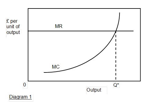
Diagram 2 presents the marginal revenue and marginal cost curves in a different way, the horizontal axis showing output measured as a reduction from the profit-maximising quantity Q*. Thus the marginal revenue and marginal cost curves are the mirror images of those in Diagram 1, and show the reductions in revenue and cost respectively from marginal reductions in output. Also shown is part of the marginal profit (MP) curve. This is simply the difference between marginal revenue and marginal cost or, equivalently, the cost in terms of lost profit of a marginal reduction in output. Given the standard continuous convex form of the marginal cost curve (a consequence of a typical U-shaped average cost curve), marginal profit will be zero when output is Q*, and the marginal profit curve will be continuous and concave (as shown).

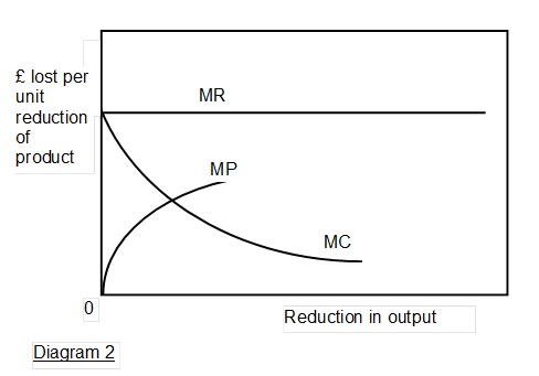
Diagram 3 shows the marginal cost of reducing emissions with output constant at Q*, so that the reduction in emissions is entirely due to technological measures. The upward-sloping form of the curve reflects the reasonable assumption that unit reductions in emissions become progressively more costly as total reductions increase. Whether the curve is linear (as shown), convex or concave will depend on circumstances. Hanley, Shogren & White suggest that it will normally be convex, but also note the possibility of economies of scale in the abatement technology, in which case it could be concave (2).

Diagram 4 shows the marginal cost of reducing emissions with constant technology, so that the reduction in emissions is entirely due to a reduction in output. In this case the cost is the lost profit, so the marginal cost curve is derived from the marginal profit curve in Diagram 2 together with the relation between output and emissions. It seems likely that in many cases the latter relation will be approximately linear. Hence the marginal cost curve is likely to resemble the marginal profit curve, albeit enlarged or reduced in the horizontal dimension to reflect the output-emissions relation.

Diagram 5 brings together the marginal cost curves of Diagrams 3 and 4. Suppose now that a per unit tax on emissions is levied at the level shown. A profit-maximising firm, applying the equimarginal principle, will reduce emissions by a combination of a reduction in output and technological measures. Relying on either method alone would mean that opportunities to reduce emissions at lower cost than paying the tax were being left unexploited. The total reduction in emissions will be that at which the marginal cost of emissions with both output and technology free to vary (the third curve in Diagram 5) equals the tax.

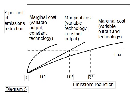
As Diagram 5 is drawn, a profit-maximising firm will reduce emissions by R* in total, of which R1 will be due to a reduction in output and R2 to technological measures. The important point here is the combination: whether more of the reduction in emissions will be due to technological measures (as shown) or more will be due to output reduction will be determined by the positions and shapes of the curves and amount of the tax, and so depend on circumstances.

There is admittedly a simplification in the above analysis. It treats the effects of output reductions and technological measures as independent, whereas in fact they influence each other. If for example output is reduced by say 10%, and this reduces emissions by 10%, then the effect of technological measures will probably be less than if output had not been reduced. This sort of interdepence is hard to show in simple diagrams. A more exact analysis might express costs and emissions as functions of both output and technology, and use differential calculus to find the profit-maximising combination for a given rate of emissions tax. Nevertheless, the implicit assumption of independence is a good approximation provided that only fairly small reductions in emissions are under consideration. And even in circumstances where the approximation is less good, the point remains that profit-maximisation in response to an emissions tax requires a combination of output reduction and technological measures.

A couple of consequences of the above are worth stating:

A larger reduction in emissions is likely, given profit-maximisation, to involve a higher proportion of the emissions reduction due to output reduction. This is a likely consequence of the concave form of the marginal cost of emissions reduction curve with technology held constant (Diagram 4). It will only not be the case if, loosely, the marginal cost of emissions reduction curve with variable technology and constant output is even more concave than that with variable output and constant technology.
A well-known piece of analysis shows that market-based instruments such as emissions taxes are more efficient than standards because they result in firms with lower marginal abatement costs contributing more to the overall reduction in emissions than those with higher marginal abatement costs (3). In the light of the above it can be seen that this principle should be broadened to relate to costs of reducing emissions with both variable technology and variable output. In particular, if two firms have available the same technology and the same output-emissions relation, then one with lower costs of reducing output, that is, the more gently sloping marginal cost and marginal profit curves, will contribute more to the reduction in emissions.

Addendum 14 June 2020

Here are the essentials of a mathematical formulation of the above. Let output be $Q$ and assume the firm is a price-taker with price $P$ per unit. Let $E$ be total emissions and let $e$ be the ratio of emissions to output, assumed constant over varying output. One could write the cost function as $C(Q,E)$ , but this would make the maths quite complicated since the partial derivative $\partial C/\partial Q$ would have no clear economic meaning: it is implausible that output could be varied while holding emissions constant. My preferred formulation is therefore $C(Q,e)$ : varying output while holding constant the emissions ratio is entirely plausible. We assume $\partial C/\partial Q > 0$ , $\partial^2 C /\partial Q^2 < 0$ and $\partial C/\partial e < 0$ .

Let $e*$ be the emissions ratio in the absence of any measures by the firm to reduce emissions, and let $Q*$ be the profit-maximising output in the absence of an emissions tax.

Now let $r(Q)$ be a reduction in output from $Q*$ , holding $e$ constant at $e*$ . The following marginal changes are associated with a marginal increase in $r(Q)$ :

Marginal change in Revenue = $-P$
Marginal change in Cost = $\partial C/\partial r(Q) = -\partial C/\partial Q < 0$
Marginal change in Profit = $-P - \partial C/\partial r(Q) = -P + \partial C/\partial Q$ (which is concave since $\partial^2 C/\partial Q^2 < 0)$
Marginal reduction in Emissions = $e*$
Marginal change in Profit per Unit Reduction in Emissions = $(-P - \partial C/\partial r(Q)) / e*$ (With varying $r(Q)$ , this corresponds to the ‘variable output’ curve in Diagram 5 above. Since the numerator is concave and the denominator is constant we can infer that the curve is concave.)

Similarly, let $r(e)$ be a reduction in the emissions ratio from e*, holding $Q$ constant at $Q*$ . The following marginal changes are associated with a marginal increase in $r(e)$ :

Marginal change in Revenue = $0$
Marginal change in Cost = $\partial C/\partial r(e) = - \partial C/\partial e > 0$
Marginal change in Profit = $- \partial C/\partial r(e) < 0$
Marginal reduction in Emissions = $Q*$
Marginal change in Profit per Unit Reduction in Emissions = $(-\partial C/\partial r(e)) / Q*$ (With varying r(e), this corresponds to the ‘variable technology’ curve in Diagram 5 above.)

Notes and References

Common M & Stagl S (2005) Ecological Economics: An Introduction Cambridge University Press p 415.
Hanley N, Shogren J F & White B (2^nd edn 2007) Environmental Economics in Theory and Practice Palgrave Macmillan pp 132-3.
See for example Hanley, Shogren & White, as 2 above, pp 133-4.