No Flood Insurance Subsidy for New UK Homes

A scheme to reduce the cost of insurance for UK homes at risk of flooding comes into effect today.  Some of the details can be criticised, but the exclusion from the scheme of new homes is absolutely right.

Flooding in parts of the UK is a fairly common event.  Winter 2015/16 brought ‘Storm Desmond’ leading to the flooding of 3,500 properties, mostly in north-west England (1).  Heavy rainfall in winter 2013/14 caused floods in several parts of southern England, Somerset being worst affected with 600 houses and much farmland flooded (2).   Other effects include disruption to transport and damage to infrastructure.  For many households, however, the most serious consequence of living in an area at risk of flooding has been the very high cost of flood insurance.

Admittedly, flooding in the UK is far less serious than in some parts of the world (3), with relatively little loss of life.  Nevertheless, flooding events such as the above always attract sustained media coverage and lead to demands for government action including immediate emergency assistance, improvements to flood protection and help to reduce insurance premiums.

If provision of insurance is left to the market, insurance companies will set premiums at levels that reflect their assessment of flood risks in particular areas, leading to very high premiums in areas of high flood risk.  Householders in such areas then face a choice between paying those premiums or leaving their property uninsured, the latter meaning that in the event of their property being flooded they would have to bear the entire cost of drying out, cleaning and repairs, and of alternative accommodation while their home was uninhabitable. They do have one other option, which is to move out of the flood risk area, but that can involve many costs and complications.  Where people have lived in an area for many years, and where the risk of flooding appears to have increased, perhaps due to climate change, it would be harsh to argue that they do not merit help because it was their choice to live in that area.

The new scheme, known as Flood Re, is the result of an agreement in 2013 between the government and insurers (4), and is underpinned by legislation (5).  Its effect will be to set a cap, at a relatively affordable level, on the flood element of buildings and contents insurance premiums.  This will mean that premiums will be much less than necessary to cover the full amount of the flood risks covered by insurers.  The difference will be funded by a tax on insurers who will almost certainly recover the cost via a small levy on all home insurance, including homes (the majority) not in areas of high flood risk.

Whether this is the best way to fund the scheme can be debated.  An alternative would be government funding from general taxation, although home insurance is so widespread that it might not make much practical difference.  Eligibility for the scheme might have been limited to people on low and perhaps middle incomes, reducing the cost to be funded.  As it is, with no income limit on eligibility, the scheme is arguably as much about supporting property markets in flood risk areas as about ensuring the affordability of flood insurance.

Another possible criticism is that the scheme will reduce the incentive for householders and local communities to try to protect themselves against flooding via measures such as keeping drainage systems in good order and not concreting over gardens and vacant land.  This is also debatable: no one would want their home to be flooded, even if fully insured; and while such small-scale measures can help, they may be less important than larger measures that may be beyond local control, such as dredging of rivers or maintenance of coastal defences.

However, an excellent feature of the scheme is that it excludes any new homes built from now on (in fact it also excludes homes built since 2009, to ensure consistency with an earlier agreement between the government and insurers (6)).  Why is this important?  Because the one certainty in this complex area is that building new homes in areas of high flood risk is bad for all concerned.  Bad for the future residents because they will have to live with the risk of flooding, even if others will bear some of the associated costs.  Bad for society generally because it will be hard for it to avoid bearing some of those costs, if only in the form of emergency help when flooding occurs.   And bad for insurers, because the risks may be hard to assess, especially in the context of climate change.  What’s more, all these bad consequences can be expected to continue for 100 years or more, the expected life of a new home.

The medical principle ‘First do no harm’ is often applicable to economic policy-making.  While environmental economists debate the finer points of taxes v marketable permits v direct regulation to limit activities that cause harm such as fossil fuel consumption, much harm around the world could be avoided simply by stopping subsidising such activities (7).  It is a merit of Flood Re that it avoids the considerable harm that would be done if the capping of insurance premiums in flood risk areas had been applied to new homes.

Notes and References

  1. Wikipedia 2015-16 Great Britain and Ireland floods https://en.wikipedia.org/wiki/2015%E2%80%9316_Great_Britain_and_Ireland_floods
  2. Wikipedia 2013-14 United Kingdom winter floods https://en.wikipedia.org/wiki/2013%E2%80%932014_United_Kingdom_winter_floods
  3. Compare for example the effects of the 2007 South Asian floods: Wikipedia https://en.wikipedia.org/wiki/2007_South_Asian_floods
  4. DEFRA (2013) Flood insurance agreement reached https://www.gov.uk/government/news/flood-insurance-agreement-reached
  5. The Flood Insurance (Scheme Funding and Administration) Regulations 2015 http://www.legislation.gov.uk/ukdsi/2015/9780111137307/contents
  6. Association of British Insurers (2008) Revised Statement of Principles on the Provision of Flood Insurance  https://www.abi.org.uk/~/media/Files/Documents/Publications/Public/Migrated/Flooding/Statement%20of%20principles%20England.pdf
  7. International Energy Agency Energy Subsidies  http://www.worldenergyoutlook.org/resources/energysubsidies/

Posted in Environment (general), Water | Tagged , | Leave a comment

Fish Stocking – A Case for Benchmarking

The performance of England’s Environment Agency in respect of fish stocking is hard to judge.  The numbers it has published don’t help very much. 

 A recent press release by England’s Environment Agency reports that in 2015 it released record numbers of coarse fish into rivers and lakes following pollution incidents or where fish stocks were low (1).  Those who like precision can read that the fish released included 53,729 chub, 46,850 dace, and so on, a total of 452,220 over nine species, plus 1.3 million larvae.  The fish were bred at the Agency’s fish breeding farm in Nottingham, and releases took place at sites across England.  This information was widely but uncritically reported in the media (2).

This is focusing on the easily measurable rather than the important.  These figures are of some use as a performance indicator for the fish breeding farm, though even in that context they need to be considered in conjunction with indicators of its unit costs and of the quality of its fish.  What they don’t indicate – and to be fair the Agency doesn’t claim that they do – is the overall performance of its fish restocking efforts, let alone of its effectiveness in fulfilling its duties in respect of fisheries and the aquatic environment.

Let’s consider what might be suitable indicators of the Agency’s fish restocking performance.  For an individual site where restocking has taken place, we are interested in whether the restocking is effective in re-establishing a self-sustaining fish population.  A possible indicator is:

Ratio of (Fish population 1 year after restocking) to (Fish population immediately before restocking)

No doubt this and the other indicators below could be refined in various ways.  Allowance might be made for: species mix; time for larvae to grow to adulthood; fish health; post-restocking incidents; and so on.  The aim here is just to identify the kinds of measures that would be useful indicators.  Where the restocking follows a pollution incident, a further indicator might be:

Ratio of (Fish population 1 year after restocking) to (Fish population before pollution incident)

For each of the above ratios, there might be assessed a threshold at which the restocking could be considered successful.  This would make possible indicators that could be calculated periodically on a regional or national basis:

Number of sites at which restocking was successful

Percentage of restocking attempts that were successful

Then there is the issue of unit costs, a possible indicator being:

(Total costs of the Environment Agency’s fish breeding and restocking operations) divided by (Number of sites at which restocking was successful)

Wherever possible, the Agency’s performance against such indicators should be benchmarked against that of other operators.  Since private fish stocking operations mainly supply fish for small private ponds, the best comparators may be public sector operators in other countries.  In the US, for example, public sector fish stocking is organised at state level, offering many potential comparators, although complications are that the species stocked differ from those in England, and more of the stocking is on a regular scheduled basis to replace fish caught and not released (3).  Benchmarking is not easy, but public bodies whose operations are largely free from the pressure of competition should attempt it, or commission benchmarking studies from specialists, to monitor their performance and identify where it falls short of best practice with a view to improvement.  They should also publish the results as part of their public accountability.

The Environment Agency’s fish restocking operation may be performing well.  I’m not aware of any evidence that it isn’t.  Equally, I haven’t found any evidence that it is. The only benchmarking study of any kind that I could find on the Agency’s websites relates to hydraulic flood models, and this appears to be an evaluation of available models which it might use, not a benchmarking of any part of its own performance (4).  Its Corporate Plan includes a ‘corporate scorecard’ listing various measures and targets, but at a fairly high level and none relating specifically to fish restocking (5).

There is a wider point here.  Environmental conservation is a serious business that isn’t helped by media reporting of simplistic numbers vaguely suggesting that something good is being done, whether they are numbers of fish restocked, numbers of trees planted, tons of material recycled, or numbers of homes powered by renewable energy facilities.  Consideration always has to be given to quality as well as quantity, consequences as well as actions, and costs – including the opportunity cost of not committing available resources to other conservation projects – as well as benefits.

Notes and References

  1. Environment Agency Press Release 11/2/2016 Almost 2 million fish released into England’s rivers  https://www.gov.uk/government/news/almost-2-million-fish-released-into-englands-rivers
  2. The BBC’s report gave additional information not in the press release. See http://www.bbc.co.uk/news/science-environment-35551906
  3. See for example Arizona Game and Fish Department Arizona Fish Stocking Schedules  http://www.gf.state.az.us/h_f/stocking_schedule.shtml  (Accessed 24/2/2016).  The ‘daily bag limits’ indicate that much fish is caught and not released, whereas in England a high proportion of angling in inland waters is on a ‘catch and release’ basis.
  4. Environment Agency: Evidence Directorate (2013) Report SC120002 Benchmarking the latest generation of 2D hydraulic modelling packages  http://evidence.environment-agency.gov.uk/FCERM/Libraries/FCERM_Project_Documents/SC120002_Benchmarking_2D_hydraulic_models_Report.sflb.ashx
  5. Environment Agency Corporate Plan 2014-16 https://www.gov.uk/government/uploads/system/uploads/attachment_data/file/402873/Environment_Agency_Corporate_Plan_2014-16.pdf  p 41
Posted in Environment (general), Fisheries | Tagged , , , , , , | Leave a comment

Time to Relax London’s Green Belt?

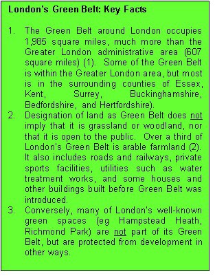
Any reform of London’s Green Belt should be informed by economic assessment of the environmental value of Green Belt land.

A feature of land use policy in the vicinity of London is the designation of large areas as Green Belt, implying a prohibition on housing and other development except in very special circumstances.  One reason why London’s housing is expensive is that demand is unconstrained except by price, while supply of a vital input – land with permission for development – is constrained by the Green Belt.

Green Belt Key FactsTwo reports published earlier this year make a case for relaxation of Green Belt.  London First’s report (3) focuses on Green Belt within the Greater London area, concluding that a small part should be released for housing development.  It proposes that land be considered for release where it is close to transport nodes and of poor environmental value (4).

The Adam Smith Institute’s report (5) focuses more broadly on Green Belts across England, but is of great relevance to London.  Its central recommendation is the abolition of Green Belt as a designation (6).  This is less radical than it may seem, because much of the most environmentally valuable land within Green Belt is protected from development by other designations including Area of Outstanding Natural Beauty and Site of Special Scientific Interest.  Having regard however to political practicability, it also suggests some alternative reforms, the most modest of which is the removal of Green Belt designation from all agricultural land within half a mile of a railway station (7).  This is quite similar to the London First proposal, albeit it would apply to the whole of the Green Belt and not just the part within Greater London.

There is considerable overlap between the arguments of the two reports.  Both point out that circumstances have changed since Green Belt was introduced in 1955.  Population has increased.  Higher incomes and wider car ownership have increased per capita demand for housing and associated off-street parking.  Both emphasize the serious consequences of high housing costs, including high proportions of many people’s income spent on housing, people on low incomes living in cramped or inadequate accommodation, inter-generational inequity, and upward pressures on labour costs jeopardizing the competitiveness of internationally-traded goods and services.

My inclination is to agree that some relaxation of London’s Green Belt is appropriate.  But there is something missing from both reports.  Neither presents any figures comparing the economic values of land for housing development and undeveloped Green Belt land.  Economic values here include not only market values but also non-market values of ecosystem services such as drainage, groundwater recharge, water purification, support for biodiversity, climate regulation, carbon sequestration and provision of green space for recreation.  If, for some Green Belt land, its value for housing development exceeds its value as undeveloped land, even when all these non-market values of undeveloped land have been taken into account, then there is an economic case for relaxation of Green Belt.  And that, surely, is the nub of the matter?  On the one hand, environmental values must be included in estimating the net benefit or cost from housing development; on the other, those values must not be treated as infinite (which is the implication of saying that a site must never be developed, come what may), but must be properly estimated by the best available methods.

However, such a comparison of values is far from straightforward.  Complications include the following:

  1. Different ecosystem services need different valuation techniques.  Some require, in the first instance, an assessment of physical or ecological effects. How much groundwater is recharged from this land?  How much carbon is sequestered by that piece of woodland?.  The chain of effects must then be traced to a point at which a credible value can be assigned, such as the cost of providing water from the best alternative source, or a recognised carbon price.  Others require revealed preference methods, eg valuing recreational green space on the basis of the travel costs incurred by visitors.  Stated preference methods (asking people how much they would be prepared to pay for an environmental service), though controversial, may also be useful.
  2. Values will differ according to location and type of land use.  The value of housing land tends to fall with distance from central London. The value of undeveloped land depends partly on location since some ecosystem services tend to be more valuable when provided close to where people live.  The nature of the undeveloped land is also important: woodland, for example, has greater value for biodiversity and carbon sequestration than some other types of land use.
  3. The value of a piece of undeveloped land is not necessarily its value in its current use.  Conversion from one type of undeveloped land to another – from arable farmland to grassland or woodland, perhaps – can increase its value, as has been shown in the UK National Ecosystem Assessment (8).  In principle, therefore, value should be value in best undeveloped use, net of any costs of conversion or transition to that use.
  4. Ecosystem services associated with housing development also need to be considered.  While blocks of flats surrounded by nothing but roads and paved areas may effectively be ‘environmental deserts’, most types of housing development in London provide some ecosystem services via gardens and local parks, which may indeed support more biodiversity than intensively cultivated farmland.
  5. The indirect effects of release of Green Belt land for housing development are also an important consideration.  Will the development of a piece of former Green Belt land result, relative to what would have occurred if that development had not taken place, in a) more housing (overall in South East England), or b) a lower average density of housing within London, or c) less housing further from London, beyond the Green Belt, or d) some combination of these?  What will be the effects on use of roads and railways, associated energy use and carbon emissions, and demand for new or improved transport links?  These indirect effects need to be valued and included (added or deducted as appropriate) in the value of land for housing development).
  6. Values may need to be adjusted to correct distortions due to taxes, subsidies and restrictions on trade. For example, the market value of farmland may exceed its economic value because of the effects of the European Union’s Common Agricultural Policy.  Adjustments may also be needed in respect of price fluctuations due to economic cycles or asset price bubbles, so as to obtain values that are not distorted by temporary circumstances.
  7. More contentiously, a case can be made that values should be weighted on grounds of equity.  If, for example, members of golf clubs are mostly well-off, a lower weighting should perhaps apply to the use values of golf courses. Carbon sequestration should arguably be given a higher weighting because it contributes to the mitigation of global climate change which poses a particular threat to people in poor countries.
  8. Allowance for future changes in circumstances is also important, conversion of land for housing being a decision with consequences for 100 years or more, and very difficult to reverse.  What population changes can be expected, and how might these impact on land values?  How might changes in transport systems and energy costs affect the trade-off many people have to make between housing and commuting costs?  Will higher world food prices or insecurity of supply increase the value of agricultural land?  Will the risk of North Sea storm surges, aggravated by climate change, eventually render some low-lying parts of London too risky for habitation?  Such considerations suggest that the land values to be compared should reflect not just current benefits but expected streams of future benefits.  They also point to a further element of value in undeveloped Green Belt land, namely, the option value implicit in retaining the opportunity for housing development at a later date.
  9. Finally (and this is perhaps the aspect that non-economists are most liable to overlook), it can be important to focus on marginal rather than total or average values.  The amount of open access grassland and woodland within London’s Green Belt is very large.  The total recreational use value of that land, reflecting (using the travel cost method) all the trips that people make to any part of it, is surely large.  But the corresponding marginal value of a particular piece of that land, that is, the recreational use value that would be lost if that piece of land were no longer available for recreational use, may be very small, unless the site is of special importance, such as a famous beauty spot, or a difficult-to-bypass section of a much-used long-distance footpath.  Most of those who would have visited or passed through that piece of land would probably visit instead a similar piece of land elsewhere, deriving similar enjoyment.

A comparison of land values which fully addresses all these complications (and others not mentioned) would be far from easy, and I am not aware of any published attempt to do so.  The National Ecosystem Assessment is of considerable relevance in that it estimates values for many kinds of ecosystem services (9), but does not directly address the question of possible conversion of Green Belt for housing.  An earlier study for the UK government by Eftec did plan to address this question by focusing specifically on the value of ‘urban fringe’ land, but was not completed (10).

The challenge is to find ways to cut through the complexity implicit in 1-9 above while obtaining results sufficiently robust to have credibility across all but the most extreme of the range of interested parties.  The following are a few ideas:

a)  It isn’t necessary to value all parts of London’s Green Belt.  Obtaining credible values for a sample of areas of agricultural land within half a mile of a railway station would take the debate a long way forward.

b)  It may not be necessary to estimate environmental values very precisely.  Suppose the value of a piece of land for housing development is estimated at £8 million per hectare (a plausible figure (11)), and its value in best undeveloped use at £100,000 per hectare.  Then it won’t matter much if the latter is so inaccurate that it should have been £50,000 or £200,000: the conclusion would be clear in any case.

c)  Values could be estimated on the basis of a set of assumptions which represents a worst case for housing development and a best case for preserving undeveloped land. Such assumptions might include a low scenario for London’s population growth, rising food prices and a rising carbon price.  If, even on such unfavourable assumptions for housing development, the value of a piece of land for housing were found to exceed its undeveloped value, the case for releasing that land for development would be strong.

Notes and References

1.     Wikipedia: Metropolitan Green Belt  https://en.wikipedia.org/wiki/Metropolitan_Green_Belt. 514,060 hectares, converted at 259 hectares per square mile.  Also Wikipedia: Greater London https://en.wikipedia.org/wiki/Greater_London [accessed 29/9/2015].

2.     Papworth T (2015) The Green Noose: An Analysis of Proposals for Reform  Adam Smith Institute (see map p 34) http://www.adamsmith.org/wp-content/uploads/2015/04/The-Green-Noose.pdf

3.     London First / Quod / SERC (2015) The Green Belt: A Place for Londoners? http://londonfirst.co.uk/wp-content/uploads/2015/02/Green-Belt-Report-February-2015.pdf

4.     As 3 above, pp 2 & 20.

5.     As 2 above.

6.     As 2 above, pp 5, 49 & 57.

7.     As 2 above, 52.

8.     Watson R & Albon S (Coordinating Lead Authors) (2011) UK National Ecosystem Assessment: Synthesis of the Key Findings p 43 http://uknea.unep-wcmc.org/Resources/tabid/82/Default.aspx   A summary was also published in Bateman I et al (2013)  Bringing Ecosystems into Economic Decision-Making: Land Use in the United Kingdom  Science  Vol 341 5 July 2013 pp 45-50 (see especially p 47).

9.     Bateman I (Coordinating Lead Author) (2011) UK National Ecosystem Assessment: Chapter 22: Economic Values from Ecosystems Table 22.27 pp 1136-8 http://uknea.unep-wcmc.org/Resources/tabid/82/Default.aspx

10.  Economics for the Environment Consultancy (Eftec) / Entec / MORI (2004)  Valuing the External Benefits of Undeveloped Land Phase 2 Vol 1 (Draft for Office of the Deputy Prime Minister)  [Accessed 29/92015 at http://www.eftec.co.uk/search-all-uknee-documents/search, entering keywords ‘External Benefits’]  This report considers the design of a contingent valuation questionnaire, but Phase 3, implementation of the questionnaire, was not pursued (source: http://www.eftec.co.uk/eftec-projects/valuing-the-external-benefits-of-undeveloped-land-phase-2-designing-a-study).

11.  Department for Communities & Local Government (February 2015) Land Value Estimates for Policy Appraisal https://www.gov.uk/government/publications/land-value-estimates-for-policy-appraisal.  Within Table 1 pp 5-12,, see especially values per hectare for land with permission for development in the following London boroughs which contain significant areas of Green Belt farmland: Bromley £10,150,000; Havering £7,300,000; Hillingdon £11,600,000.

Posted in Cities | Tagged , , , , , | Leave a comment

Signal and Noise in the Oil Market

Conventional wisdom has been that cost of finding and extracting oil is on a secular rising trend.  Given the current low price of oil, is that still credible?

A famous saying attributed to Keynes was his challenge to a critic: “When the facts change, I change my mind.  What do you do, sir?” (1).  In the global oil market, a key fact has changed.  The price of a barrel of oil, which had been around $110 from 2010 to mid 2014, fell during the latter part of 2014 to around $50 and, if futures markets are to be believed, even by 2020 will still be below $70 (2).

Doesn’t this show that all that fuss about peak oil, scarcity and rising costs was wide of the mark?  The function of prices, after all, is to allocate scarce resources: a fall in the price of a resource surely implies that it has become less scarce?

Let’s take this step by step.  How will owners of operational oil wells respond to a reduction in price from $110 to $50?  In most cases they will continue extracting oil at more or less the same rate, because their unit operating costs (including royalties where applicable) are generally below $50 (3,4).  Oil production involves large exploration and construction costs, but once a well becomes operational these costs have already been incurred, so are irrelevant to the decision to continue production.  A price of $50 may accelerate the closure of some ageing wells with high operating costs.  The main impact of such a price, however, will be to discourage investment in new exploration and construction, bringing about a reduction in future oil supply.  In summary, oil supply is price-inelastic in the short run, but price-elastic in the long run.

Similar considerations apply on the demand side.  Car owners or those with oil-fired heating will increase their oil consumption only a little in response to even a large price reduction, because their consumption is largely determined by their needs and the particular vehicles or heating systems they have.  Only when they come to buy a new car or boiler is a low price likely to have a major impact on their behaviour (making them less concerned about fuel-efficiency than they would be if the price were higher).  Demand, too, is therefore price-inelastic in the short run, but price-elastic in the long run.

The price of oil at any time is determined by the equilibrium of short-run supply and demand.  Why?  Because in a largely free global market, buyers and sellers can rapidly exploit any mis-match between supply and demand.  By so doing, they ensure that the price rapidly adjusts  to restore equilibrium.  Restoration of equilibrium requires changes in quantity supplied and/or demanded, and these are achieved within a timescale far too short for investment in new productive capacity or replacement of consumer durables to be of relevance.

Diagram 1 below shows, on the left, the cost structure of a typical firm, and on the right, supply and demand in the global market (the output axis on the right is to a much smaller scale).  The short-run average cost curve (SAC) shows the firm’s average costs given its current capital stock and rights to oil reserves, and from it is derived the short-run marginal cost curve (SMC), which is also its short-run supply curve.  The sum of the short-run supply curves for all firms is the global short-run supply curve (SS), and this together with short-run demand determines the price of oil.  Two not very different demand curves (SD1 and SD2) are shown, resulting, because of the inelasticity of both supply and demand, in very different prices P1 and P2.  Similarly (not shown in the diagram) a small shift in the supply curve with constant demand can result in a large change in price.

Oil Diagram 1

Diagram 1 also shows the firm’s long-run average cost (LAC) curve, which assumes the optimum capital stock for each level of output. This is in red to highlight its importance: in the long run the firm can be profitable only if the price of oil generally exceeds average cost.  Looking at it another way, the firm will not invest in exploration and construction unless it expects the future price of oil to exceed long-run average cost.  The important point to note, as illustrated by P1 and P2, is that price at any time can be either much more or much less than long-run average cost.

A price well above or below long-run average cost can always be explained, with hindsight, in terms of past under- or over-investment.  Investment in increased productive capacity tends to shift the global short-run supply curve to the right, reducing price.  However, the forecasts of supply and demand on which firms base their investment plans may prove inaccurate for various reasons including new technologies, gamesmanship by major producers (eg OPEC), disruptions to supply, recessions and changes affecting competing energy sources.  The relationship between the price of oil at any time and its long-run average cost of production is mediated by the productive capacity of the global oil industry, and for all these reasons it is difficult for the industry to get this right.

The price of oil at any time, therefore, tells us little about long-run average costs.  The recent fall in price is quite consistent with a gradual increase in the cost of finding and extracting oil as the more accessible reserves are exhausted.

But is it actually the case that the long-run average cost of producing oil is rising, and likely to go on rising?  To answer this, it helps to distinguish between conventional and unconventional oil, although definitions of these terms vary (5).  Here I take conventional oil to be oil that can be extracted using traditional drilling methods from beneath land or shallow water.  Such oil is becoming increasingly difficult to find (6).  Even if it remains relatively cheap to extract where it can be found, its share of total oil production has declined, and is likely to decline further.

Unconventional oil – including tight oil (sometimes termed shale oil), oil sands and deep-water oil – contributed more than two-thirds of the increase in total oil production between 2000 and 2012 (7).  Its share of total oil production will probably continue to increase as conventional oilfields are exhausted.  Although each type of unconventional oil has its own characteristics, extraction costs are generally high, with break-even costs per barrel estimated at $65 for US tight oil, $75 for Canadian oil sands and $95 for deepwater oil (8).

In terms of long term trends in the oil market, the fall in price to $50 is just noise.  The real signal is the effect it has had on firms’ investment plans.  ExxonMobil is cutting its capital spending in 2015 by 12% (9), BP by about 20% (10), Conoco by 35% and Occidental by 33% (11).  That is a strong indication that much previously planned investment would only be profitable at a price well above $50.  That is what really does tell us something about average costs.  So it remains highly credible that the cost of producing oil is continuing on an upward trend.

Notes and References

  1. Quite possibly a mis-attribution. See  http://quoteinvestigator.com/2011/07/22/keynes-change-mind/
  2. CME Group: Crude Oil Futures Quotes http://www.cmegroup.com/trading/energy/crude-oil/light-sweet-crude.html  [Accessed 5 April 2015]
  3. Schoen J W (12/1/2015) When, and where, oil is too cheap to be profitable CNBC  http://www.cnbc.com/id/102326971
  4. Udland M (11/12/2014) Here is a Simple Way of Seeing Who Gets Screwed Most as Oil Tumbles  Business Insider UK  http://uk.businessinsider.com/oil-cash-costs-2014-12
  5. Wikipedia: Unconventional oil http://en.wikipedia.org/wiki/Unconventional_oil#Defining_unconventional_oil
  6. Reuters (17/2/2014) Global Oil Firms Seen Cutting Exploration Spending Fox Business  http://www.foxbusiness.com/industries/2014/02/17/global-oil-firms-seen-cutting-exploration-spending/?utm_source=feedburner&utm_medium=feed&utm_campaign=Feed%3A+foxbusiness%2Flatest+%28Internal+-+Latest+News+-+Text%29
  7. Dancy J (12/11/2013) IEA: The Shale Mirage – Future Crude Oil Supply Crunch?  Financial Sense  http://www.financialsense.com/contributors/joseph-dancy/iea-shale-mirage-future-crude-oil-supply-crunch   (first paragraph of section headed ‘All Liquids Are Not Equal’)
  8. Yep E (4/11/2014) Falling Prices May Choke Off Energy Flows to Asia  The Wall Street Journal  http://blogs.wsj.com/moneybeat/2014/11/04/falling-prices-may-choke-off-energy-flows-to-asia/
  9. Yahoo News (4/3/2015) ExxonMobil cuts spending but predicts higher output  http://news.yahoo.com/exxonmobil-cuts-capital-spending-falling-oil-prices-150140256.html
  10. Yahoo News (3/2/2015) BP cuts investment as sliding oil hits profit  https://uk.news.yahoo.com/bp-cuts-investment-sliding-oil-082111522.html#gXQert1
  11. Macalister T & Monaghan A (29/1/2015) Shell slashes spending and calls for North Sea tax cuts   The Guardian  http://www.theguardian.com/business/2015/jan/29/shell-cuts-spending-oil-price-slide  (see paragraph above Price of Oil chart re Conoco and Occidental

Posted in Energy | Tagged , , , , , , , , | Leave a comment