Differences in national rates of Covid-19 infection may be partly due to differences in household sizes.
While many questions about the Covid-19 virus are currently unanswered, one point on which there has been wide agreement is that transmission is more likely indoors than outdoors (1,2). If therefore we are to explain differences in national rates of infection, an obvious place to look is differences in indoor environments. A plausible hypothesis is the following:
Rates of Covid-19 infection will be higher, other things being equal, in larger households, that is, households with more occupants.
The thinking behind this is simple. If one member of a household becomes infected, and unless there is effective self-isolation within that household, then it is quite likely that their infection will transmit to other members. The larger the household, the more people they can infect. The hypothesis does not imply that household size is the sole or main reason for differences in rates of infection, merely that it is one contributory factor.
If correct, the hypothesis suggests a possible link between housing policy and rates of Covid-19 infection. Countries (such as the UK) with restrictive planning policies that have limited the supply of land for building new homes will have fewer homes than they would otherwise have. This reduced supply of housing will lead to higher costs (whether for ownership or renting). As a consequence, fewer people will be able to afford their own home, and (other things being equal) average household sizes will be larger: young adults, for example, will tend to stay longer with their parents before setting up their own home. Larger households in turn will create more scope for transmission of infection.
But is the hypothesis correct? An ideal test would require large sample data on household size and numbers infected at individual household level. Here I present the results of a ‘quick and dirty’ test based on data currently available at national level.
At the present time, reliable data on total rates of infection since the start of the outbreak is not available. National totals of confirmed cases are incomplete because many cases have not been confirmed by testing, and international comparisons of those totals reflect differences in rates of testing as much as in rates of infection. I therefore used national rates of death from Covid-19 as an, admittedly imperfect, proxy for rates of infection. Even such death rates are unlikely to be perfect for international comparison, since practice in recording the cause of death of patients with multiple conditions may vary. As a proxy for rates of infection, death rates suffer from the limitation that they are also influenced by differences in health systems between countries. Nevertheless, it seems reasonable to assume, at least for the developed countries of Western Europe, that official figures on deaths from Covid-19 are at least of the right order of magnitude.
Average household size was calculated from national statistics for population and numbers of households.
A regression was estimated for the model:
DP = C + (B x PH) + E
where: DP is death rate from Covid-19 per million population; C is the regression constant; B is the slope coefficient; PH is average population per household; and E is the error term. The regression was run on data for 14 Western European countries: Austria, Belgium, Denmark, France, Germany, Italy, Ireland, Netherlands, Norway, Portugal, Spain, Sweden, Switzerland, United Kingdom.
Estimation of the regression was by weighted least squares, with weighting by population (implying that the fitting of the regression line takes more account of data points for countries with larger propulations). The justification for the weighting is that a local random factor affecting the death rate within a region with a population of a few million could have a large effect on the overall death rate of a country with a smaller population. Within a larger country, however, the effect of such a local factor would be less, and different random factors within different regions of the country would probably tend to offset each other. It is proper to record that the choice of weighted least squares, rather than ordinary (ie unweighted) least squares, makes a large difference to the result.
The estimated regression line was:
DP = -1,334 + (770 x PH)
The precise values of the estimated coefficients, which rather implausibly imply a nil death rate at a household size of about 1.7, are not important. What does matter is that the estimated slope coefficient is positive, consistently with the hypothesis (and is sufficiently large that the null hypothesis that its true value is zero or less is rejected at the 5% significance level (3)).
I would describe this result as ‘interesting’. But no more conclusion should be drawn than that the hypothesis merits further research.
A spreadsheet containing the underlying data and full regression output may be downloaded here:
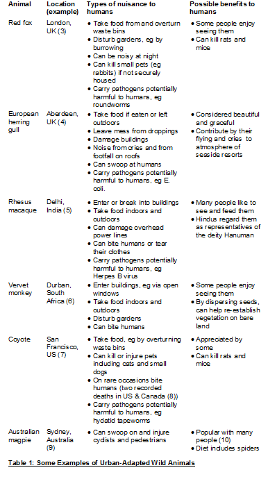
In many cities around the world, there are wild animal species whose presence is enjoyed by some and a nuisance to others. Management of such species should be informed by economic analysis as well as ecological, ethical and animal welfare considerations.
I had better say this right away: this post was prompted not by the current Covid-19 pandemic, but by repeated sightings last summer of a fox around my London home. Nevertheless, the pandemic does show that the proximity of wild animals can in certain circumstances have enormous adverse consequences for humans. At the time of writing, the precise source of the initial outbreak in Wuhan, China, is not known, but it appears that the virus was transmitted from wild animals to humans at a market. Quite possibly, however, it was a wild animal farmed outside the city and brought to market for sale, and not therefore urban wildlife in the sense considered in this post.
Human attitudes to wildlife depend greatly on its nature, location and behaviour. Large carnivores in what remains of their natural habitats are widely considered worthy of conservation efforts, but if such a creature should be on the loose in a city, as happens occasionally (1), then most people would support its killing in the interests of public safety if other options are impractical or ineffective. Very small animals encountered in or near people’s homes may evoke little affection or sympathy: many who would never harm larger animals will happily swat a fly or lay a mouse trap.
Between these extremes are medium-sized wild animals present in and adapted to life in cities about which people may have differing or complex attitudes – animals not large or dangerous enough to present a major physical risk to human life, but capable of being a considerable nuisance while also evoking human sympathy and the protection of custom or law. Table 1 below lists some examples (this has been compiled from numerous online sources which it would be tedious to list in full).
Trying to be objective, I have avoided any reference to animals “attacking” humans, as it is apparent that what one source considers an attack, another may view as defensive action in response to human provocation or to protect young. In the same spirit, I have not stated that any of the animals “spread” human diseases. Undoubtedly many urban wild animals carry pathogens that are potentially harmful to humans (2). The questions then are the likelihood of transmission to humans, and whether transmission can be prevented by simple precautions such as washing hands after contact or requires more elaborate preventive measures. It is also pertinent to consider whether or not the risks to humans are greater than those already encountered from pets and domestic animals.
There seems to be little literature on the application of economics to the management of such urban wildlife. What literature there is on the economics of wildlife management focuses mainly on rural wildlife, as is apparent from the highlighting of costs from harm to livestock and crops, and benefits from hunting and recreation (11). Nevertheless, the insight that there may exist an optimum population size which maximises benefits less costs (12) appears relevant to urban as well as rural wildlife.
Before pursuing this argument, I will briefly address some lines of thought that seem unlikely to be helpful in informing management strategies for species of the sort listed in the table. Firstly, conservation is not normally an issue for such species. It may be that their adaptation to urban environments is to some extent a response to loss of their natural habitats. But all the listed species are classified by the International Union for the Conservation of Nature as of least concern (13), implying that their populations are large enough that they are far from any risk of extinction. Secondly, and as a consequence of the above, a focus on such species’ contribution to biodiversity, and on the economic value of that contribution, is unlikely to yield useful information. There is no foreseeable risk that that contribution will be lost.
Any attempt to measure the benefits and costs to humans of an urban wildlife species would require application of a judicious selection of non-market environmental valuation techniques. Benefits from observing animals might be measured by adapting the travel cost method, typically used in valuing parks and other recreational sites, to allow for the fact that the animals are not concentrated at one site but spread out across an urban environment. Thus the relevant travel costs are not those incurred in getting to a particular site but those incurred in getting to wherever, at a particular time, an animal can conveniently be observed. The “travel” required to make such an observation when at home might be no more than getting up and coming to a window when alerted to an animal’s presence by a family member. The fact that such “travel” may involve very little cost – the value of perhaps just a minute or two of a person’s time – does not mean that the benefit is correspondingly low. This is because the travel cost method measures value in terms of consumer surplus – in simple terms the difference between the cost a person would have been willing to incur to view an animal and the cost they actually incur. The cost they would have been willing to incur might be assessed from the costs actually incurred to view an animal by other people who happen to live where such animals are not present.
Benefits from controlling species regarded as harmful might be measured using a combination of ecological and economic analysis. Ecological analysis would attempt to quantify the effect of the population of the beneficial species on the population of the harmful species, and the relation between the population of the harmful species and specific forms of harm (theft of unprotected food, dispersion of pathogens, dropping of faeces, chewing of materials, etc). It would then be for suitable economic analysis to attempt to value the benefit from a reduction in the relevant forms of harm.
The costs attributable to urban wildlife include numerous components. Theft of food that would otherwise have been available for human consumption can as a minimum be costed at its market value or, where prepared at home from bought-in ingredients, at the market value of the ingredients plus the opportunity cost of the preparation time. The cost of overturned bins might be taken to be the opportunity cost of the time spent in cleaning up, and that of disturbance to gardens and damage to buildings the cost of reinstatement or repair. In the case of damage to overhead power lines, the cost of the power outage should be added to the repair costs. Power outage costs will depend on how many users are affected and what they use electricity for, but can be very large (14). The cost of injury or ill-health attributable to urban animals should include the costs of associated healthcare and of lost income (to employees) or lost production (to employers) due to time off work. Given suitable information about the effect of education on children’s employment and earnings prospects, one might also include a cost element for time off school. Estimating the costs of ill-health of retired people raises issues beyond the scope of this post (15).
Where nuisance attributable to animals is recurrent, further costs may arise. Various forms of avertive behaviour may be adopted in an effort to minimise the nuisance. These may include: never eating out of doors; keeping windows closed (even in hot weather); buying larger or more secure waste bins; fitting spikes where birds might want to perch; setting deterrents such as motion-sensitive lights, chemical sprays and imitation snakes; and going out of one’s way to avoid certain locations. All these have costs: either direct monetary outlays, or time costs, or costs of restrictions on life-style. The last-named costs might be estimated using the hedonic property method, requiring comparison of house prices in locations with and without the need for such restrictions.
None of this is easy. Even an apparently simple case such as theft of purchased food requires reliable data on the quantities and types of stolen items, and the species responsible for theft. Although the economics of environmental valuation has made great strides in recent decades, its application to the full range of benefits and costs of particular species, and collection of the necessary data, would present enormous challenges.
It is plausible to suppose that a higher urban population density of a wild species will not imply proportionately higher benefits to humans. The principle of diminishing marginal utility suggests that someone who enjoys seeing a fox or a monkey is unlikely to obtain ten times as much enjoyment from seeing ten foxes or monkeys, or from seeing just one ten times as often. That could be tested empirically by observing how much time and effort a person incurs to view such animals, and how that time and effort varies with the number of known opportunities for views.
The costs to humans of a higher urban population density of a wild species, however, may be more than proportionately higher. One overturned waste bin in a street may be seen as an exception. Many such bins not only create proportionately more clean-up work, but may also be perceived as lowering the tone of the neighbourhood, and may prompt efforts to address the problem by deterrent measures or obtaining more animal-proof bins. Occasional animal noises may be a minor issue, but persistent noise, especially at night when it may disturb sleep, can be a serious problem. Similarly, occasional theft of food may be tolerable, but routine thieving may force changes in life-style, such as never eating out of doors, keeping windows closed even in hot weather, and abandoning businesses selling food at outdoor market stalls.
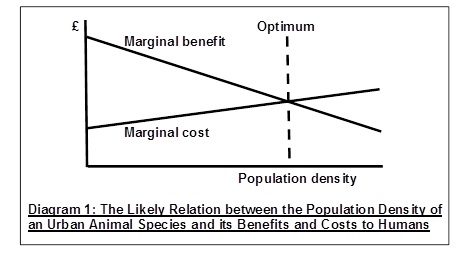
If these suggestions are broadly correct, then we can represent the situation in terms of the sort of diagram familiar from, for example, the economics of pollution control.
As in other contexts, net benefit is maximised when marginal benefit equals marginal cost.
However, such an approach should not be the sole determinant of how a species should be managed. It is also important to consider, from the perspectives of effectiveness, cost and ethics, the means of getting from the current to the optimum population. More fundamentally, an animal rights perspective would suggest that an approach based solely on benefits and costs for humans is to be rejected as an example of human supremacism (16).
What would be missing, in an approach that only takes account of benefits and costs for humans, is consideration of animal welfare. That implies, as a minimum, avoidance of direct cruelty to animals including, in particular, avoidance of practices such as blocking of dens and use of poisons that subject animals to lingering and unnecessarily painful deaths. The importance of animal welfare in this narrow sense is widely recognised: in the UK, for example, use of such practices to kill foxes is illegal (17).
However, appropriate management of urban wildlife requires a much broader conception of animal welfare that has regard to the extent to which animals lead worthwhile lives with a positive balance of well-being over suffering, and to how humans and the urban environment they create can affect that balance. Positive features of an urban habitat may include a plentiful food supply and an absence of natural predators. Negative features may include intense competition for territory and the risk of death or injury in road accidents. The balance might be expected to vary between species and locations.
Ideally, management of an urban species should be informed by knowledge not only of the actual welfare of its members but also of how their welfare might change if its population density were to increase or reduce, or if features of its environment were to change. But rarely if ever do we have such knowledge (18). Even our knowledge of actual welfare is very limited.
There is a further difficult and contentious issue. Philosophers have explored, in respect of humans, the ethics of policies that affect the size of the future population. How should we choose between scenarios A and B, if people in A have greater well-being but people in B are more numerous? Totalism asserts that we should maximise total well-being, calculated as population multiplied by average quality of life (19). Averagism holds that we should maximise average quality of life, without regard to size of population. Both these positions, and others, have been shown to have counter-intuitive implications. A considerable literature in this field has not led to anything approaching a consensus. The point here is this: the same ethical issue arises in respect of actions or policies which affect the size of an animal population.
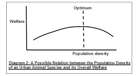
A plausible assumption is that the average well-being of an animal species is greatest when its population density is neither too small nor too large. If it is too small, then it may be very difficult for individuals to learn behaviour from others or to find mates. If it is too large, then competition for territory may become severe, diseases may spread more easily, and the available food supply may be inadequate. Rather more speculatively, it might be argued that if population expands beyond the level that its food supply can support, then average well-being will decline so rapidly as to render the debate between totalism and averagism irrelevant (because total welfare will fall despite the extra population). If so, then the relation between population density and welfare, according to whatever is our preferred measure of overall welfare of an animal population, could be represented as in the diagram below.
There is still much that this analysis leaves out. It passes over the issue of what in an animal’s environment we are regarding as held constant as its population density varies. Whatever management method might be chosen – for example shooting, poisoning or sterilization for a reduction in population, and providing extra food or nesting opportunities for an increase – would in itself amount to a change in the environment. It also omits the ecological consequences of a change in the population density of an animal species. Through food chains and in other ways, there are likely to be effects on the populations of other animal species, and so in turn on the welfare of those species.
Nevertheless, it is I believe of interest to consider the implications of putting together the economic analysis summarised in Diagram 1 and the animal welfare analysis summarised in Diagram 2. I assert the following:
Proposition 1: There is no reason to suppose that the population density of an urban animal species that optimises its net benefit to humans is the same as, or even close to, the population density that optimises its own overall welfare.
The justification for Proposition 1 is simply that the bases of the optimum for humans and the optimum for the animal species are entirely different. It would be entirely coincidental if these optima happened to be the same or close.
For the next proposition it is convenient to represent the actual current population density of an urban animal species in a particular location as A, its optimum density for humans as OH, and its optimum density for animal welfare as OA. We can then state:
Proposition 2: For any urban animal species, there are 6 possible orderings by increasing animal population density of A, OH and OA. For 4 of these orderings, there is available what might be termed a Pareto improvement (20), a change in population density that would yield a net benefit for humans and raise the overall welfare of the animal species. For the other 2 orderings, a change in animal population density that was advantageous to humans would be disadvantageous to the animal species, and vice versa.
The 6 possible orderings are: 1) A < OA < OH ; 2) A < OH < OA ; 3) OA < OH < A ; 4) OH < OA < A ; 5) OA < A < OH ; 6) OH < A < OA .
For ordering 1, an increase in population density from A to OA would optimise the overall welfare of the animal species, but also bring the net benefit for humans closer to that at OH. For ordering 2, an increase from A to OH would optimise for humans but also raise overall welfare for the animal species. For orderings 3 and 4, a suitable reduction in population density would be beneficial for both humans and the animal species. It is only for orderings 5 and 6, in which A is between OA and OH, that a change in density can be beneficial for humans or for the animal species, but not for both.
Proposition 2 should not be taken to imply that the 6 orderings are equally likely: such a claim would be way beyond what can be supported by current knowledge. What it does suggest, however, is that, in the management of an urban animal species there is not necessarily a conflict between what is good for humans and what is good for the species. Where an urban animal species is, on balance, a nuisance to humans, it is possible that a reduction in its population would also be good for the species.
However, that is just a possibility. It is also possible that a reduction in the population of an urban animal species would be good for humans but bad for the species. Much more research is needed to enable us to make well-supported decisions on the management of urban animals.
See for example Gren I-M, Haggmark-Svensson T, Eloffson K & Engelmann M (2018) Economics of Wildlife Management – an overview European Journal of Wildlife Research 64:22 https://link.springer.com/article/10.1007/s10344-018-1180-3 – start of Introduction
See for example Gren et al as 12 above, p 3
This can be confirmed at the IUCN Red list website https://www.iucnredlist.org/, entering in turn the names of the species.
See for example Huter K et al 2016 Economic evaluation of health promotion for older people – methodological problems and challenges BMC Health Services Research 16 (Suppl 5) https://www.ncbi.nlm.nih.gov/pmc/articles/PMC5016726/
I use the term Pareto improvement here in a specialised sense. It is not implied that such a change would leave each individual human and each individual animal no worse off, only that overall welfare for humans and overall welfare for animals would both be improved.
The economic
theory of public goods is sometimes assumed to be adaptable in a
straightforward manner to public bads. Here
I consider some implications of the fact that such bads are usually mitigable.
Consider a region around an airport, subjected to noise from
flights. Noise arrives at every home in
the region, but any household can choose, at a cost, to moderate the noise
level inside its home by installing double glazing. Such a choice by a household has no effect on
the noise level inside any other home.
Suppose the sole water supply to a poor village is
polluted. Everyone in the village will
be risking their health if they drink that water as supplied. But (for some types of pollutant) any household
can treat its water to make it safer to drink, perhaps by filtering or chemical
treatment. Such a choice by a household
has no effect on the safety of the water consumed by any other household.
Similarly, suppose a region’s agriculture is affected by a
drought. All farms in the region receive
less rainfall than normal but some, because of the crops they have chosen to
grow or their cultivation methods, are better able than others to withstand the
effects of the drought. Such choices by a farm have no effect on the resilience
of other farms.
These are all examples of what I call mitigable public bads. The idea
of a public bad is derived from that of a public
good, commonly defined as a good which is both rival and non-excludable. By
non-rival is meant that one person’s consumption of
or benefit from the good does not reduce the amount available to others.
Non-excludable means that neither the provider of the good nor any other agent
is able to pick and choose which individuals within the scope of provision of
the good can consume it (hence the free-rider
problem consisting in the fact that those who decline to pay for the good
cannot be excluded from benefiting from it).
Street lighting in a city, for example, is non-excludable because no one
can determine that certain individuals passing through the city’s streets will
have their way illuminated and others will not. The fact that the provider
could turn off the lights, excluding everyone, is irrelevant, as is the fact
that only those who live in or visit the city can benefit from its street
lighting.
Public
bads have sometimes been defined as “goods” which are non-rival and
non-excludable but which tend to lower rather than raise welfare (1). For a bad to be non-rival is usually clear
enough: my disturbance by noise from flights does not render my neighbours’
disturbance any less. But non-excludability
in relation to a bad is not so clear. No
one can be expected to pay for a bad, so a “provider” such as a factory causing
air pollution has no interest in excluding non-payers. And whereas it can be
assumed that few would wish to exclude
themselves from a public good, sufferers from a public bad will certainly
so wish if they can do so at reasonable cost.
Usage in this context seems not to be settled.
But I find it convenient to use the term public
bad for any welfare-lowering “good” which is both non-rival and, in the
sense that no one can pick and choose who within its broad scope suffers from
it and who is excluded, non-excludable. If affected
individuals can take action to moderate the effects of the bad on themselves,
then I shall say that the public bad is mitigable.
Environmental economists sometimes refer in this context to defensive expenditure or avertive expenditure, but as an
adjective qualifying public bad, my
sense is that mitigable is more
appropriate than defensible or avertable. Mitigable public bads are thus a subset of
public bads, but an important one, as the above examples suggest. Indeed, it seems plausible that most public bads are mitigable, at least
for some individuals and to some degree.
Mitigation need not be limited to individuals
acting alone. In the case of installing double glazing, a decision by a
household, or by a group of households making a bulk purchase to obtain a
discount on the installation cost, can still be regarded as mitigation. But for most public bads a clear distinction
can be made between mitigation, action
by potential sufferers to protect themselves from the bad, and what I shall
term reduction, consisting in action
at or close to the source of the bad to limit its scale or scope. Examples of reduction would be a ban by an
airport authority on flying to and from the airport in a certain direction,
limiting noise for all households in that direction, or installation of
equipment by a smoke-emitting factory to capture pollutants in the smoke,
improving air quality for everyone in its vicinity.
Two
more definitions will be useful. I shall refer to the state of a public bad as its condition, across the whole of the
affected region, after any reduction but before consideration of possible
mitigation. By an individual’s exposure
I shall mean the condition of the bad as experienced by that individual after any mitigation they have
undertaken. Thus exposure can differ
between individuals both because some parts of the affected region may be
affected more badly than others, and because the mitigation they have
undertaken may differ.
A
well-known result concerning public goods can be stated informally as below:
Proposition 1 The level of provision of a public good is optimal if the marginal cost of providing the good equals the sum over individuals of their marginal benefit from the good.
An individual’s marginal benefit from a public good can be interpreted
as their marginal rate of substitution of the good for private goods. This is equivalent to the slope of an indifference
curve connecting combinations of goods which yield the individual the same
utility. Since an individual’s utility function defines a whole set of
indifference curves, the question then is which
curve’s slope should be included in the sum when we are considering a possible
re-allocation of production between private goods and the public good. The
answer I will rely on here is to take the status
quo distribution of private goods between individuals and assume that, in
any re-allocation of production, individuals’ quantities of private goods would
all change pro rata to the total
quantity of private goods. Any quantity
of the public good together with an individual’s implied quantity of private
goods would then define a point identifying a single indifference curve of that
individual. An alternative approach is
to assume that all the indifference curves of any one individual have the same
shape and therefore the same slope at any one quantity of the public good,
regardless of the individual’s quantity of private goods. This is equivalent to assuming that
individual utility functions are quasilinear in the private goods (2), and is
plausible if the quantity of private goods that individuals would have to forgo
in return for the public good is small in relation to the total private goods. Under this assumption it does not matter
which curve of each individual we take: the sum of the slopes of one curve per
individual will be the same whichever curves we take.
A point
quite properly highlighted in most discussions of public goods is the sharp
contrast between Proposition 1 and the optimality condition for a private good, which requires that the
marginal cost of provision equal each
individual’s marginal benefit. From this it follows that a public good will be
under-provided in a free market (3). However,
other features of the proposition are sometimes overlooked. Firstly, the idea
of optimal provision makes no sense for natural
public goods like sunshine, except to the extent that they can be manipulated
by human intervention. Secondly, for those cases where optimal provision does
make sense, it is often a gross oversimplification to assume that the level of
provision can be adequately characterised as a number of units on a single
scale. Just consider national defence, commonly
given as an example of a public good. Thirdly, the relevant marginal cost of
providing the public good is marginal social
cost. In the case of street lighting,
for example, marginal cost should include the marginal social cost due to any
greenhouse gases emitted in generating the electricity to supply the lights.
Having
noted these points, which apply equally to public bads, we may ask what is the
equivalent of Proposition 1 for a mitigable public bad. In this case there are
two kinds of decision to be made: the extent of mitigation by each individual;
and the extent of action at source to limit or reduce the bad.
Given
the state of the bad, a rational individual will undertake mitigation up to but
not beyond the point at which their marginal cost of mitigation (MCM) equals
their benefit from a marginal lessening of exposure (BMLE). This is assuming
normally shaped curves, that is, marginal cost increases and marginal benefit
falls with additional units of mitigation.
For the purpose of optimal mitigation by individuals, it is not
important how units of mitigation and exposure are defined: the only
requirement is that, for any one individual, marginal cost and marginal benefit
are measured with respect to the same units.
Note that, even if mitigation is possible for an individual, they will
not undertake any mitigation if their marginal cost at zero mitigation exceeds
their marginal benefit at that point. In symbols, the condition under which an individual will
undertake mitigation is:
MCM0 <
BMLE0 (A)
where the zero subscript indicates that the marginal quantities
are measured at the state of the bad.
By
analogy with the case of a public good, we expect that for a state S of a bad
to be optimal, the marginal cost of reducing S must equal the sum over
individuals of some sort of marginal quantity.
But what exactly? The benefit to
an individual from a marginal reduction in the state (BMRS) will depend upon
whether, at S, they will undertake mitigation. If inequality A is not satisfied
so that they do not undertake mitigation, then their benefit from a marginal
reduction in S is simply their benefit from a marginal lessening of exposure:
BMRS(MCM0 > BMLE0) = BMLE0 (B)
If
however inequality A is satisfied so that they undertake mitigation, then their
net benefit from mitigation at the margin will be BMLE minus MCM. Hence their
benefit from a marginal reduction in S is the benefit from a marginal lessening
of exposure less the benefit they
could instead have obtained themselves from mitigation, the difference being
the marginal cost of mitigation:
Proposition 2 Provided individual mitigation behaviour is rational, the state of a mitigable public bad is optimal if the marginal cost of reducing the bad equals the sum over individuals of the lower of a) their benefit from a marginal lessening of exposure and b) their marginal cost of mitigation.
However, extreme care is needed to ensure consistency in the units
of measurement of the various marginal quantities. Suppose we have a defined scale on which to
measure the state of a bad. For each
individual, units of exposure must be such that the harm suffered from u units of state together with
sufficient mitigation to limit exposure to u
– 1 units must be the same as the harm suffered from u – 1 units of state with no mitigation. A unit of mitigation is then simply that
quantity of mitigation which will reduce exposure by one unit.
This has the important implication that both the physical
requirements for and the cost of a unit of mitigation may vary greatly between
individuals according to their circumstances.
Suppose the state of noise in the region around an airport is measured
by average loudness at a defined location near the airport. A given number of units will then be
associated with more noise at some locations than others. Suppose, as may be the case, that noise falls
off with distance from the airport. A
reduction of one unit in the state of the noise may be quite significant for
someone living close to an airport, but barely noticeable for someone on the
edge of the affected region. Consequently the latter would need to do less than
the latter, in physical terms, to achieve one unit of mitigation, and their
marginal cost of mitigation will be lower.
Notwithstanding the above, a person living further from the
airport will be less likely than someone nearer to it to undertake mitigation
if, as is likely, benefit from a marginal lessening of exposure falls even
faster with distance than marginal cost of mitigation, eventually reaching a point
at which further lessening is imperceptible and offers no benefit.
The public policy implications of Proposition 2 are that those
mitigable public bads which are due to human activity tend to be over-provided
in a free market, but also that the extent of government action to correct that
market failure should have regard to the availability and cost of mitigation by
individuals. If for example a tax is the
preferred policy instrument, then it would be sub-optimal if the chosen tax
rate per unit of state exceeds the sum over individuals as defined in
Proposition 2.
An important question now is how the optimal state of a mitigable public bad compares with what it would be if no mitigation were possible. This is illustrated in Chart 1 below.
The
horizontal axis shows the state of the bad, reducing (ie improving) from left
to right. The vertical axis shows the
quantity of a composite good representing all private goods. It is assumed that there are no other public
bads and no public goods. The production
possibility frontier PPF is the outer boundary of the possible combinations of
the public bad and private goods, its concave shape reflecting the standard
assumption of a diminishing marginal rate of transformation between goods. The status
quo is assumed to lie somewhere on the PPF.
S is the optimal state on the assumption that mitigation is
impossible, and line I is the sum of individual indifference curves on the same
assumption, chosen as explained above. The
slope of I at S will be the sum over individuals of their BMLE’s at S, and given
the status quo assumption, I will be
tangent to the PPF.
The red line IM is a sum of indifference curves passing through
the intersection of PPF and I, on the assumption that mitigation is available. If
inequality A above were not satisfied for any individual so that no mitigation would
be undertaken, the slope of IM at S would also be the sum over individuals of
their BMLE’s at S, and IM would be coincident with I in the vicinity of S,
which would still be optimal despite the availability of mitigation. If however A is satisfied for at least some
individuals so that mitigation is undertaken, then the slope of IM will be a
sum which includes MCM for at least some individuals, and therefore less than
the slope of I. Hence there is a region
to the left of S within which PPF meets curves higher than IM, and the optimal
state, given mitigation, will lie within this region, perhaps at SM. So we have:
Proposition 3 Provided individual mitigation behaviour is rational, the optimal state of a public bad for which mitigation is available is greater (ie worse) than or equal to what the optimal state would have been if mitigation were not available, and is strictly greater if at least some individuals would have undertaken mitigation at the latter state.
In
developing here a theory of mitigable public bads, I have passed over several
points suggesting that Propositions 2 and 3 are in need of qualification. Without following through the implications of
each, I will just mention that an individual’s private cost of mitigation may
not equal the social cost (for example the manufacture of double glazing may
involve external costs not reflected in its price), that mitigation expenditure
may be taxed or subsidised, and that rational mitigation behaviour may involve
an element of gamesmanship if individuals believe that mitigation may lead to
less action by government to reduce a bad.
It also needs to be borne in mind that optimality does not imply an
acceptable income distribution: sometimes considerations of equity can properly
take precedence over optimality.
Environmental
valuation studies should be clearer as to whether the value they estimate is
marginal value or something else.
The idea of a marginal quantity is one of the most-used in
the economist’s toolkit. In the theory of
the firm, profit is maximised when marginal revenue equals marginal cost. In macroeconomics, the effect of a change in
disposable income depends on the marginal propensity to consume. In the literature on valuation of non-market
environmental goods, however, this tool seems not to be used as often as it
should. Travel cost studies estimating
the value of recreational sites often fail to consider whether what they have
estimated is the marginal or some other value of the site, and this can lead to
inappropriate policy recommendations.
The sense of marginal value with which I am concerned here
is that which considers a whole recreational site as one unit. Admittedly that could raise a difficulty in
respect of open countryside with no clear subdivisions, but for urban parks surrounded
by developed land and for designated national or country parks with
well-defined boundaries it is usually clear enough. So I am not concerned with the difference in
value between a park as it is and the same park with one less square metre of
land. The margin I mean is that between
the status quo in respect of all the parks in a region and a situation with one
less park. One might argue that incremental would be a more correct
term, but I consider that marginal
has connotations that are relevant here, such as the idea of diminishing
marginal utility.
A couple of examples will illustrate why it matters whether or
not the value estimated by a study is marginal value. Suppose there is a proposal
to convert a recreational site for housing development, which we want to
evaluate by cost-benefit analysis. This
involves, for both costs and benefits, comparing the situations with and
without the project (1). The
recreational value that should be used in the analysis is therefore a marginal
value, the value that would be lost if the site were no longer available for
recreational visits. If there are other
recreational sites in the vicinity, then people who would have visited that
particular site might visit other sites instead. If so, then the numbers of visits to the
particular site and the costs incurred by its visitors will not give a good
guide to the value that would be lost. It
should of course be borne in mind, here and throughout this post, that
recreational value is only one component of the total economic value of
undeveloped land – others include the values of water and air purification,
biodiversity and carbon sequestration -, and decisions on land use conversions
should have regard to all such components.
Sometimes, however, marginal value is not the value we
need. Suppose we want to include the
value of a recreational site in the national accounts, as part of an estimate
of the aggregate value of the country’s environmental assets or natural
capital. In that case the marginal value
is not appropriate. Suppose two sites A and B are not far apart. If we value site A on a marginal basis,
excluding the value attributable to visitors who would have visited site B if
site A had not been available, and if we apply the same approach, vice versa,
when valuing site B, then we will not capture the full combined value of the
two sites. In simple terms, the value
attributable to visitors with no strong preference between the sites will be
missed.
How then should we estimate the marginal recreational value
of a park? And where marginal value is
not what we want, what other value concepts are available and how should they
be estimated? A key consideration here
is that parks are not a homogeneous good: they differ in location, size and
other characteristics. This has several
implications. We should not expect a
smooth curvilinear relation between the number of parks in a region and their
combined value. Obtaining the marginal
value of a park is certainly not a matter of estimating such a curve and then applying
differential calculus. Each park will
have its own marginal value. Furthermore,
the average value of a park, obtained by dividing the total value of the parks
in a region by the number of parks, is unlikely to be a useful statistic.
To address the above questions, I shall consider the example
below of a stylised small town with two parks.
The grey zone C2 is the commercial and shopping centre, with
no residents. The two green zones B2 and
E1 are parks with free entry, also without residents. The remaining seven zones are residential,
each with the same number of residents: what the number is does not matter as
all my calculations were per resident.
In the interests of simplicity I make the following
assumptions:
All residents are alike in their behaviour in respect of park visits. Their visit rates depend only on the travel costs of their visits to parks.
Residents perceive the two parks as different but equally attractive, except in so far as visits require different travel costs.
Distances are measured as straight lines between the centres of zones, the unit of distance being the side of one square zone.
The travel cost (TC) of a resident’s visit to a park is measured in monetary units such that it equals the park’s distance from the resident’s zone.
There are no complications arising from congestion or multi-purpose trips.
I pass over the important practical question, a key focus of
attention in many published studies, of how the formulae modelling visit rates
(trip-generating functions) might be estimated from observational data. My focus here is on the determination of site
values from the trip-generating functions, and I therefore start from plausible
assumptions about those functions. By
plausible I mean that the functional forms are credible; the coefficient values
are chosen so that all residents will make some
visits to each park, but their visit rates will vary considerably depending
on their zone of residence.
It is convenient to define the functions in two stages. The first stage consists of formulae stating
what the visit rate to a park would be if, hypothetically,
the other park were not available (to indicate the hypothetical nature of these
visit rates I write VR’). These formulae
are:
The formulae for actual visit rates, given the availability
of both parks, are then expressed in terms of these hypothetical visit rates:
The formula for VR(E1) is as above but with B2 and E1
interchanged throughout. These formulae
may appear complicated, but are chosen for various desirable properties
(further details are in the download at the end of this post). Note that a simple linear functional form as below
will not work:
While it correctly indicates that a higher travel cost to
park E1 will be associated with a higher visit rate to park B2, it has the very
implausible implication that the relation between VR(B2) and TC(E1) is
linear. The higher TC(E1) is, the
smaller we would expect the effect on VR(B2) of a unit increase in TC(E1) to be.
To calculate values, starting from these trip-generating
functions, I applied the standard method of deriving points on the demand
curves by considering various price additions to the travel cost, then taking
the area under the demand curve (the consumer surplus) to be the value (2). Applying this method to the actual
trip-generating functions, I obtained values per resident of 21.66 for park B2 and 16.06 for park E1, implying a total
value of 37.72. An appropriate description for these values
would be “contribution of visits to the park to the total value of the two
parks”. This (generalised to all the
parks in a country) is the value concept that would be relevant for inclusion
in the national accounts as above.
The lower value for park E1 – the more distant park for more
than half of the residents – is unsurprising, notwithstanding the equal
attractiveness of the two parks. There
is much evidence that the recreational value of sites is lower when they are
further from centres of population, other things being equal (3).
I also applied the method to the hypothetical trip-generating functions, obtaining values per resident (in each case in the absence of the other park) of 28.26 for park B2 and 22.26 for park E1. This enabled the marginal values to be obtained as follows (calculations may not exactly agree due to rounding:
Marginal value of park B2
=
(Total value of two parks) less (Value of park E1 in absence of park
B2)
= 37.72 – 22.26 = 15.45
Marginal value of park E1
=
(Total value of two parks) less (Value of park B2 in absence of park
E1)
= 37.72 – 28.26 = 9.45
The table below summarises these results.
Total value is shown only for the “contribution” row: totals of the other rows would not be meaningful.
Once one has both the actual and the hypothetical
trip-generating functions, the calculations of these distinct values do not
present any special difficulty. Why then
do published travel cost valuation studies often fail to consider whether the
values they obtain are marginal values or contributions to total value?
One possible reason is that researchers may not be entirely impartial. They may be seeking results that would support a case for preservation of a site, and recognise that a marginal value, which could be low, would not be helpful. Certainly, I have seen quite a few such studies that use their results in recommending preservation, perhaps with the help of government funding. I cannot however recall a single study concluding that a site was not worth preserving.
Another reason is that many studies, perhaps because of resource limitations, focus on a single site. They may, with the aim of avoiding omitted variable bias, estimate a trip-generating function that includes travel costs to alternative sites as independent variables. But even then, it is impossible to obtain the marginal value of a site from a trip-generating function for that site only. As we have seen above, that requires such functions for other sites too.
Suppose however that a researcher is both impartial and
well-supplied with resources. Suppose
that they collect data on visit rates and travel costs for a number of sites in
a region. They could then estimate the
actual trip-generating function for each site and hence calculate each site’s
contribution to total value. To obtain
the marginal value of a site, however, they would still have to estimate the hypothetical trip-generating functions
describing the unobservable visit
rates to other sites that would prevail if that site were unavailable. That seems, at best, statistically
challenging.
It is understandable, therefore, that many studies lead to value estimates for a site that are a reasonable approximation to “contribution to total value”, but do not estimate, even approximately, the marginal value. What is less defensible is when such values are used to justify policy recommendations, for example whether a site should be preserved or converted to an alternative land use, that really require the marginal value. One such example is a paper by Bharali & Mazumder (2012) which estimates the recreational value of Kaziranga National Park, Assam, India (4). Starting from sample data on visit rates, travel costs and other relevant variables, the authors obtain an estimate of consumer surplus which, they state, “signifies the value of the benefits that the visitors derived from visiting the park” (5). But they do not consider whether those benefits are gross, or net of the benefits that visitors would have obtained at alternative sites if the park had not been present. Since the paper does not consider alternative sites at all, we can take it that these benefits are gross and that the value it estimates is not marginal value. Nevertheless, the author’s conclude that the government should allocate large funds to preserve the site (6). That conclusion would be much better supported if it had been shown that the marginal value of the site were significant.
The calculations underlying the above results may be downloaded here: Marginal Park Value Calculation (MS Excel 2010 format).
See for example Perman R, Ma Y, McGilvray J & Common M (3rd ed’n 2003) Natural Resource and Environmental Economics Pearson Addison Wesley pp 413-4
See for example Bateman I et al (2013) Bringing Ecosystem Services into Economic Decision-Making: Land Use in the United Kingdom Science Vol 341 Issue 6141 pp 45-50 (section headed National-Scale Implications) http://science.sciencemag.org/content/341/6141/45
Bharali A & Mazumder R (2012) Application of Travel Cost Method to Assess the Pricing Policy of Public Parks: the Case of Kaziranga National Park Journal of Regional Development and Planning Vol 1(1) pp 41-50 http://www.jrdp.in/archive/1_1_4.pdf
Bharali & Mazumder, as 4 above, p 47. An unusual feature of this paper (an error?) is that, having estimated the consumer surplus, it then adds on the actual travel costs to arrive at what it describes as total recreational value.