In the absence of full cost information or of externalities, should policies to support production of a good always be technology-neutral? Scenarios can be constructed which suggest not, but the gains from departing from technology neutrality may be too small to be worthwhile.
Suppose a government wishes to secure the production of a good which can be produced by more than one technology. It might be a good required by the government sector, or one required by firms or households which the government wishes to subsidise because it supports its social or environmental policy. Should the government proceed in a technology-neutral manner, or could it be appropriate to favour one technology over another? There are some circumstances in which the latter approach is clearly better. One is where the government has full information on the production costs of the different technologies, so can choose the technology or combination of technologies offering the lowest cost. Another is where the apparently similar goods obtained from the different technologies are not actually identical, an example being intermittent electricity obtained from sources such as wind and solar on the one hand, and continuous electricity (subject only to maintenance requirements and faults) obtained from nuclear on the other. A third is where the technologies differ in respect of production externalities: again electricity provides an example via the contrast between generation from fossil fuels and from low-carbon sources.
Suppose however that none of these circumstances apply: in other words the government has less than full information on costs, the alternative technologies produce goods which are genuinely identical, and there are no production externalities. I want to consider a line of reasoning suggesting that a technology-neutral approach may still not be best. This post is largely prompted by a paper by Fabra & Montero (1), although I shall present the material in my own way and draw my own conclusions.
In the interests of simplicity, I shall assume that the quantity 


To illustrate these two interpretations of ‘best’ and how they can be achieved, let us flesh out our scenario with sufficient detail to permit the use of mathematical optimisation techniques. Let us assume that the government must pay the same unit price for all amounts of the good produced using a technique, but can discriminate in respect of price between the two techniques. Let the quantities produced using the two techniques be 

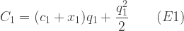
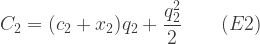
Costs here are taken to include normal profit, so we can assume that a firm will produce if and only if the unit price offered by the government equals or exceeds its unit cost. At aggregate level, therefore, the quantity of the good produced by a technique will be such that the aggregate marginal cost (4) equals the price offered:


Suppose further that the government knows the above formulae and knows the values of 


![[-k, k],](https://s0.wp.com/latex.php?latex=%5B-k%2C+k%5D%2C&bg=ffffff&fg=333333&s=1&c=20201002)


To determine the unit price(s) the government should offer, it clearly needs to undertake some sort of auction process. I shall consider five possible types of auction, setting out the relevant maths in some detail for the first and in outline for the others (5).
An immediate question is whether the government should hold separate auctions for the two techniques or a single auction embracing both. I will consider the separate auctions (technology-specific) case first. This requires the government, using only the information it has, to determine the optimal quantities to be obtained by use of each technique. Because some of its information is stochastic, it needs to consider the expectation, denoted 
If the aim is to minimise cost to the government, the problem can be formulated as:
![\min E[p_1q_1+p_2q_2]\qquad(E5)](https://s0.wp.com/latex.php?latex=%5Cmin+E%5Bp_1q_1%2Bp_2q_2%5D%5Cqquad%28E5%29&bg=ffffff&fg=333333&s=1&c=20201002)
Since we require 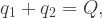

![\min E[c_1+x_1+q_1)q_1+(c_2+x_2+Q-q_1)(Q-q_1)]\qquad(E6)](https://s0.wp.com/latex.php?latex=%5Cmin+E%5Bc_1%2Bx_1%2Bq_1%29q_1%2B%28c_2%2Bx_2%2BQ-q_1%29%28Q-q_1%29%5D%5Cqquad%28E6%29&bg=ffffff&fg=333333&s=1&c=20201002)
Given that the distributions of the variables ![E[x_1] = E[x_2] = 0,](https://s0.wp.com/latex.php?latex=E%5Bx_1%5D+%3D+E%5Bx_2%5D+%3D+0%2C&bg=ffffff&fg=333333&s=1&c=20201002)
![E[x_1x_2] = E[x_1]E[x_2] = 0,](https://s0.wp.com/latex.php?latex=E%5Bx_1x_2%5D+%3D+E%5Bx_1%5DE%5Bx_2%5D+%3D+0%2C&bg=ffffff&fg=333333&s=1&c=20201002)
![E[x_1^2],](https://s0.wp.com/latex.php?latex=E%5Bx_1%5E2%5D%2C&bg=ffffff&fg=333333&s=1&c=20201002)
![E[x_2^2],](https://s0.wp.com/latex.php?latex=E%5Bx_2%5E2%5D%2C&bg=ffffff&fg=333333&s=1&c=20201002)

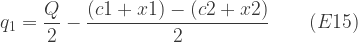
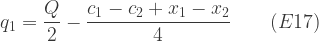
![\min [2q_1^2+(c_1-c_2-2Q)q_1 + c_2Q + Q^2]\qquad(E7)](https://s0.wp.com/latex.php?latex=%5Cmin+%5B2q_1%5E2%2B%28c_1-c_2-2Q%29q_1+%2B+c_2Q+%2B+Q%5E2%5D%5Cqquad%28E7%29&bg=ffffff&fg=333333&s=1&c=20201002)
Differentiating with respect to

implying (7):

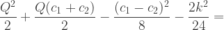
Substituting our known values we have 

![E[p_1q_1+p_2q_2]=E[(130+x_1)30+(90+x_2)70]=](https://s0.wp.com/latex.php?latex=E%5Bp_1q_1%2Bp_2q_2%5D%3DE%5B%28130%2Bx_1%2930%2B%2890%2Bx_2%2970%5D%3D&bg=ffffff&fg=333333&s=1&c=20201002)

where, again, we can ignore terms containing
![E\Big[(c_1 + x_1)q_1 + \dfrac{q_1^2}{2} + (c_2 + x_2)q_2 + \dfrac{q_2^2}{2} + 10,200 \lambda \Big]](https://s0.wp.com/latex.php?latex=E%5CBig%5B%28c_1+%2B+x_1%29q_1+%2B+%5Cdfrac%7Bq_1%5E2%7D%7B2%7D+%2B+%28c_2+%2B+x_2%29q_2+%2B+%5Cdfrac%7Bq_2%5E2%7D%7B2%7D+%2B+10%2C200+%5Clambda+%5CBig%5D&bg=ffffff&fg=333333&s=1&c=20201002)
![= E\Big[(100 + x_1)30 + \dfrac{30^2}{2} + (20 + x_2)70 + \dfrac{70^2}{2} + 10,200(0.2)\Big]](https://s0.wp.com/latex.php?latex=%3D+E%5CBig%5B%28100+%2B+x_1%2930+%2B+%5Cdfrac%7B30%5E2%7D%7B2%7D+%2B+%2820+%2B+x_2%2970+%2B+%5Cdfrac%7B70%5E2%7D%7B2%7D+%2B+10%2C200%280.2%29%5CBig%5D&bg=ffffff&fg=333333&s=1&c=20201002)

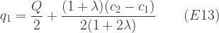
To obtain this outcome, the government must proceed by what I shall call Auction Type 1:
Invite bids from technique 1, and set the strike price at the level just sufficient to bring forth production at the level (
It is important to note that this procedure (and all the others to be considered) only works because of our assumption that there are many small firms with a range of production costs. Because of this, we can take it that each firm’s bid reflects its actual costs. A firm can gain nothing from a higher bid since, with many small firms, such a bid cannot significantly raise the strike price, but can (if the bid exceeds the strike price) result in the firm losing the business it could have gained.
If the aim is to maximise welfare, which as we have seen requires minimising economic cost, the problem is formulated as:
![\min E\Big[(c_1 + x_1)q_1 + \dfrac{q_1^2}{2} + (c_2 + x_2)q_2 + \dfrac{q_2^2}{2} + \lambda (p_1q_1 + p_2q_2)\Big]\qquad(E12)](https://s0.wp.com/latex.php?latex=%5Cmin+E%5CBig%5B%28c_1+%2B+x_1%29q_1+%2B+%5Cdfrac%7Bq_1%5E2%7D%7B2%7D+%2B+%28c_2+%2B+x_2%29q_2+%2B+%5Cdfrac%7Bq_2%5E2%7D%7B2%7D+%2B+%5Clambda+%28p_1q_1+%2B+p_2q_2%29%5CBig%5D%5Cqquad%28E12%29&bg=ffffff&fg=333333&s=1&c=20201002)
Substituting as before for 
Substituting known values we have
To obtain this outcome, we require Auction Type 2:
Invite bids from technique 1, and set the strike price at the level just sufficient to bring forth production at the level (
A feature of both the approaches we have considered is that, given our known values, they result in different prices for electricity according to the technique by which it is produced. Suppose instead that the government holds what we will call Auction Type 3:
Invite bids from techniques 1 and 2, and set a single strike price at the level just sufficient to bring forth total production at the required level
= 100).
In this case, from E3 and E4 we can infer:

implying:
Although we can infer formulae for 
This type of auction does not achieve the best outcome on either of our interpretations of ‘best’. It results in an expected cost to the government higher than either Type 1 or Type 2, and an expected economic cost higher than Type 2. What it does minimise, by equalizing the prices and therefore the marginal costs of production using the two techniques, is the total production cost. But that is not what we want to minimize under either of our interpretations of ‘best’.
It may come as a surprise that the government can do better than any of the approaches considered so far. The key here is that the government can hold a single auction without committing itself to set a common strike price. This is sometimes termed a product mix auction (8), the principle being applicable to differentiated goods or to a common good that can be produced in more than one way. Given that, based on our assumptions, each firm’s bid reflects its actual costs, the set of bids received in an auction provides the government with a lot of cost information. It can use that information to choose strike prices for each technique according to its aim.
If the aim is to minimise the cost to the government, the problem to be solved after holding the auction is:

Proceeding as above, albeit without needing at this stage to consider the expectation, we obtain:
Note that we do not ignore the terms in

For purpose of comparison with our earlier results, especially from Auction Type 1, we want the expectation of E18 over the range of possible values of

We can also calculate the expectation of the economic cost which is 9,326.
For this expected outcome we require Auction Type 4:
Invite bids from techniques 1 and 2, and using the results of the auction, set the strike prices for each technique at levels which a) are just sufficient to bring forth total production
If the aim is to minimise economic cost, the problem to be solved, again after holding the auction, is:
![\min \Big[(c_1 + x_1)q_1 + \dfrac{q_1^2}{2} + (c_2 + x_2)q_2 + \dfrac{q_2^2}{2} + \lambda (p_1q_1 + p_2q_2)\Big]\qquad(E20)](https://s0.wp.com/latex.php?latex=%5Cmin+%5CBig%5B%28c_1+%2B+x_1%29q_1+%2B+%5Cdfrac%7Bq_1%5E2%7D%7B2%7D+%2B+%28c_2+%2B+x_2%29q_2+%2B+%5Cdfrac%7Bq_2%5E2%7D%7B2%7D+%2B+%5Clambda+%28p_1q_1+%2B+p_2q_2%29%5CBig%5D%5Cqquad%28E20%29&bg=ffffff&fg=333333&s=1&c=20201002)
Proceeding as above, this can be solved to obtain:

The expected cost to the government is 10,604 and the expected economic cost is 9,037. These expected outcomes are achieved by Auction Type 5:
Invite bids from techniques 1 and 2, and using the results of the auction, set the strike prices for each technique at levels which a) are just sufficient to bring forth total production
Table 1 below summarises the above results.
| Auction type | 1 | 2 | 3 | 4 | 5 | |
| Minimising | Cost to govt | Economic cost | Cost of production | Cost to govt | Economic cost | |
| No. of auctions | Separate auction for each technology | Single auction embracing both technologies | ||||
| Pricing | Price for each technology | Common price | Price for each technology | |||
| Cost to govt | 10,200 | 10,608 | 11,000 | 10,192 | 10,604 | |
| Economic cost | 9,340 | 9,054 | 9,083 | 9,326 | 9,037 | |
What can be inferred from these results?
Firstly, the classification of auction types reveals an ambiguity in the term ‘technology-neutral’. Should we reserve that term for type 3 with a single auction and a single strike price? Or should we also include types 4 and 5, the product-mix auctions, on the grounds that they have a single auction embracing both technologies? The assertion is often made that climate change policies should be technology-neutral, often I suspect without awareness of the possibility of a product-mix auction.
Secondly, the choice of aim is important. Comparing auction types 1 and 4 on the one hand with types 2 and 5 on the other, the former result in the cost to government being c 400 (3.8%) lower, while the latter result in the economic cost being c 300 (3.2%) lower.
Thirdly, although the product-mix auctions 4 and 5 give the best results, the gains they offer relative to the best alternatives are very small, at least given the parameter values in our central case. Focusing on expected economic cost, type 5 yields an advantage of only 17 (0.2%) over type 2. Table 2 below shows the effects on expected economic cost of various changes in parameters, variation 0 being our central case. Variations 1-3 show that changes in
| Auction type | 2 | 3 | 5 | |
| Variation | ||||
| 0 | c2 = 20; k = 10; λ = 0.2 | 9,054 | 9,083 | 9,037 |
| 1 | c2 = 20; k = 10; λ = 0.1 | 7,987 | 7,983 | 7,970 |
| 2 | c2 = 20; k = 10; λ = 0.0 | 6.900 | 6,883 | 6,883 |
| 3 | c2 = 20; k = 10; λ = 0.4 | 11,158 | 11,283 | 11,140 |
| 4 | c2 = 20; k = 18; λ = 0.2 | 9,054 | 9,046 | 8,999 |
| 5 | c2 = 50; k = 10; λ = 0.2 | 11,857 | 11,858 | 11,840 |
| 6 | c2 = 50; k = 40; λ = 0.2 | 11,857 | 11,608 | 11,583 |
It can be seen that type 5 is superior to types 2 and 3 in all cases except variation 2, when with
Given that a product-mix auction may be perceived as introducing additional complexity for limited benefit, it is of interest to compare the outcomes of type 2, the technology-specific approach, and type 3, the technology-neutral common price approach. Looking at variations 0 and 4, and then at 5 and 6, it can be seen that, other things being equal, changes in
Comparing variations 0, 1, 2 and 3, it can be seen that the relative outcomes of types 2 and 3 are also affected by
Conclusion
We have considered a limited range of scenarios. Alternative scenarios might include any or all of the following features: more than two available techniques; different production functions; larger firms with scope for gamesmanship; government providing subsidies rather than meeting full costs. The sorts of results we have obtained might not carry over to all scenarios.
However, it has been shown that, if a technology-neutral auction is taken to mean an auction with a common strike price for different techniques for producing the same good, it will not necessarily yield more economic welfare than a technology-specific auction. For the scenarios considered, however, the advantage of the technology-specific auction is very small given likely ratios of the excess burden of tax to the direct burden.
It has also been shown that a suitably designed product-mix auction, which can be considered technology-neutral in the sense that a single auction embraces alternative techniques, can achieve more economic welfare than any other auction type. However, the advantage over the best alternative auction type, in all the cases we have considered, is rather small.
Although the single auction common price approach is generally sub-optimal, from a welfare perspective it is no more than very slightly sub-optimal in any of the cases we have considered, except that in which the excess burden of tax ratio is very high. This suggests that a government aiming to maximise welfare may be unlikely to go far wrong with a technology-neutral approach.
Our most significant finding is a rather obvious one. Whether the auction type is technology-neutral or technology-specific, the choice of aim matters. An auction designed to minimise cost to the government will result in a sub-optimal outcome from a welfare perspective. Equally, an auction designed to maximise welfare will mean a higher cost than necessary to the government. The difference in both cases may be of the order of 3-4%.
Notes and References
- Fabra N & Montero J-P (2022) Technology Neutral vs. Technology Specific Procurement MIT Centre for Energy and Environmental Policy Research https://ceepr.mit.edu/wp-content/uploads/2022/03/2022-005.pdf See especially pp 6-15
- Wikipedia – Excess burden of taxation https://en.wikipedia.org/wiki/Excess_burden_of_taxation
- For a more formal specification of the relation between firm-level and aggregate production costs see Fabra & Montero, as 2 above, p 6
- Obtained by differentiating E1 and E2 with respect to q1 and q2 respectively.
- Readers familiar with elementary algebra and calculus should be able, from the information given, to confirm all my results, although the algebra is in some cases rather tedious.
- Wikipedia – Continuous uniform distribution – Moments https://en.wikipedia.org/wiki/Continuous_uniform_distribution#Moments See formula for second moments and put a = -k, b = k.
- To confirm that this value of q1 corresponds to a minimum, note that the second derivative is 4 > 0.
- The idea appears to be due to Paul Klemperer: see the first version (2008) of his paper on the topic at https://www.nuffield.ox.ac.uk/economics/papers/2009/w6/BoeTarp28_7_09.pdf
- Browning E K (1976) The Marginal Cost of Public Funds Journal of Political Economy Vol 84(2) p 283 https://www.jstor.org/stable/1831901
- Harrison G W, Rutherford T F & Tarr D G (2002) Trade Policy Options for Chile: The Importance of Market Access The World Bank Economic Review Vol 16 No. 1 p 57 https://documents1.worldbank.org/curated/en/760701468001806330/pdf/35057.pdf
- Auriol E & Warlters M (2009) The Marginal Cost of Public Funds and Tax Reform in Africa Toulouse School of Economics Working Paper Series 09-110 https://www.tse-fr.eu/sites/default/files/medias/doc/wp/dev/wp_dev_110_2009.pdf