In Defence of the Linear Demand Function

Presentations of microeconomic analysis often assume linear demand functions, but rarely justify them in terms of utility theory. However it can be done, and without making outrageous assumptions.

Originally posted 11/2/2016. Re-posted following site reorganisation 21/6/2016.

Run a Google search on “assume a linear demand function”, and you get thousands of hits. The straight-line demand function is much used in elementary economic analysis and student exercises, presumably because the complexities of curves can distract from a topic’s economic substance, perhaps even just because it’s easy to draw. But is there more to be said for it than that? Could a real demand function be linear?

The answer to the question might seem to lie in empirical investigation, and certainly that could be helpful. For the most part, we would have to rely on natural experiments in which the price and other variables have changed through the normal working of an economy, and use statistical methods to try to isolate the effect of the price. Given some unexplained variation in the data points, the form of the demand function may be far from clear.

Furthermore, the range of prices observed may be quite narrow. The fitted demand function may be of doubtful value if we want to predict the effect of a price outside that range, or to use the consumer surplus (the area under the whole demand function above the actual price) as a welfare measure. The latter point is especially important in the economic valuation – from revealed preferences in surrogate markets – of environmental goods for which the actual price is often zero. The travel cost and hedonic methods often require measurement of the area under the whole demand function for an environmental good, right down to zero price, so that it becomes crucial to consider the shape of the demand function even at very low prices.

There remains therefore a considerable role for theory, in particular utility theory. While theory cannot tell us the form of the demand function for a particular good, it can provide some insight into what forms are possible, and in what sort of circumstances they might occur. A general principle of econometrics is that model-building should be supported by theory (1), and the identification of demand functions is no exception.

The derivation of a demand function from a utility function together with a budget constraint is a straightforward application of constrained optimisation. The converse – to find the utility function that will result in a given form of demand function – needs more mathematical sophistication. A detailed treatment, including the case of linear demand, may be found in Border (2). The utility function developed below, leading to a linear demand function, is an adaptation of that derived by Border. The aim here is to show that such a utility function is not just a mathematical curiosity, but in certain circumstances has economic plausibility.

Let’s consider some utility functions, for the case of two goods, X and Y. Take the functions to relate to a normal person, neither rich nor with an unusually modest desire for goods. To relate the two-good case to the reality of a world of many goods, take X to be a particular good in whose demand function we are interested, and Y to be a composite good representing all other goods. Suppose further that X is an inessential, a leisure good for example. Let $P_X$ and $P_Y$ be the prices of the goods, with $P_Y$ assumed fixed, and let M be the person’s income.

The assumption that more of a good is normally preferred to less suggests two basic types of utility function, multiplicative and additive. To allow some degree of flexibility, we may include coefficients in either type, say a and b, leading naturally to the two forms below:

$U(X,Y) = X^aY^b\qquad(E1)$

$U(X,Y) = aX + bY\qquad(E2)$

The multiplicative approach results in the familiar Cobb-Douglas utility function (E1). A feature of this function is that it exhibits a diminishing marginal rate of substitution, represented by indifference curves that are convex to the origin. In other words, as we increase the quantity of one good, say X, the ‘value’ of given increments gradually decreases, where value is measured in terms of the quantity of Y that must be forgone to keep utility constant. A standard piece of analysis (3) shows that it leads to curvilinear demand functions with demand inversely proportional to price, implying that there is no limit on quantity demanded as price falls to zero. These properties suggest that the Cobb-Douglas function may be plausible in some circumstances. For our case, however, it is inappropriate because it implies that utility will be nil when consumption of X is nil, even if consumption of Y is high, which contradicts the assumption that X is an inessential.

What is needed for our case, therefore, is an additive utility function. However, the basic additive form (E2) exhibits perfect substitutability between the two goods, represented by straight-line indifference curves. If we increase the quantity of X in this case, the value of given increments, in terms of the quantity of Y that must be forgone to keep utility constant, does not decrease. Since this is not very plausible, let us refine (E2) by replacing aX and bY by functions f(X) and g(Y):

$U(X,Y) = f(X) + g(Y)\qquad(E3)$

To ensure a diminishing marginal rate of substitution, we require that, as X and Y respectively increase from zero, these functions initially increase, but at a decreasing rate (in terms of calculus their first derivatives are positive and their second derivatives negative).

Since X is an inessential good, we expect that the rate of increase of f(X) will decrease quite rapidly, so that f(X) will reach a maximum at quite a low threshold value of X, and will remain at that maximum when X exceeds the threshold. For the composite good Y, however, we expect that the rate of increase of g(Y) will decrease much more slowly, and that g(Y) will still be increasing at the maximum Y the individual can afford from their income, that is, $M/P_Y$ .

The indifference map will look something like that below, although the relative sizes of the horizontal and vertical dimensions will depend on the units in which the goods are measured and the scales of the axes.

Any expenditure on X above that needed to achieve the threshold will not add to the utility derived from X, and by reducing expenditure on Y will reduce the utility derived from Y. A rational individual will therefore spend most (or all) of their income on Y and at most a very small proportion q on X.

The possible range of expenditure on Y will therefore be small, implying a narrow range for consumption of Y:

$M(1-q)/P_Y \leq Y \leq M/P_Y\;(E4)$

Since the rate of increase of the Y component g(Y) of U decreases only very slowly, a straight line can provide a very good approximation of g(Y) within the narrow range defined by (E4), narrow because q is very small. Hence we can find parameters, say s and t, such that within the defined range:

$s + tY \approx g(Y)$

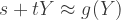
We can therefore rewrite (E3), to a very good degree of approximation within the relevant range, as:

$U(X,Y) = f(X) + s + t(Y)\qquad(E5)$

It remains to consider the function f(X). A simple way to achieve the necessary properties – increasing in X, but at a decreasing rate – is:

$f(X) = aX - cX^2\qquad(E6)$

It can be seen (eg using differentiation) that f is increasing when X is less than $a/2c$ , and comes to a maximum of $a^2/4c$ at that threshold (when X exceeds the threshold we assume that it remains at that maximum, rather than declining as (E6) suggests).

There are other functions that share the same properties. For example, the square in (E6) could be replaced by a cube, or some other power, and if desired the parameters a and c could be calibrated to yield the same maximum as (E6). However, such functions differ in their curvature, a simple indicator of which is the ratio R of their value at half the threshold to their value at the threshold (their maximum). For (E6) we have:

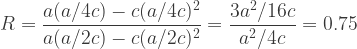
$R = \dfrac{a(a/4c) - c(a/4c)^2}{a(a/2c) - c(a/2c)^2} = \dfrac{3a^2/16c}{a^2/4c} = 0.75$

It can be shown that the higher the power replacing the square in (E6), the lower R becomes. For a cube, for example, it is about 0.69. While there cannot be said to be a correct value of R, which may vary between individuals and between goods, a value of three-quarters for a leisure good – implying that a person gets three-quarters of the possible enjoyment from half the quantity at which they are sated – seems entirely plausible.

For the circumstances we have described, therefore, a plausible form of utility function within the relevant range is:

$U(X,Y) = aX - cX^2 + s + tY\qquad(E7)$

We now use the standard constrained maximisation technique to find the demand function for X. The budget constraint is:

$XP_X + YP_Y = M$

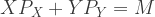
Hence the Lagrangian expression is:

$L(X,Y,\lambda) = aX - cX^2 + s + tY + \lambda(XP_X + YP_Y - M)$

Taking partial differentials and equating to zero:

$\partial L / \partial X = a - 2cX + \lambda P_X = 0$ s=1$

$\partial L / \partial Y = t + \lambda P_Y = 0$

Hence:

$\lambda = (2cX - a)/P_X = -t/P_Y$

$2cX = a - tP_X / P_Y$

$X = (a/2c) - (t /2cP_Y)P_X\qquad(E8)$

Since a, c, t and by assumption $P_Y$ are all constant, the demand function (E8) is linear in $P_X$ .

A caveat. The above is an individual demand function, and like all demand functions is subject to the overriding condition that demand cannot be negative. Because of that condition, a market demand function built up by summing linear individual demand functions is not necessarily linear along its whole length. This is only so where each individual demand function has the same choke price (lowest price at which demand is zero). Otherwise, the market demand function is linear over the price range from zero up to the lowest choke price of any of the individual functions, but will be kinked at that choke price (and at all higher individual choke prices).

Notes and References

Gujarati D N (International Edition 2006) Essentials of Econometrics McGraw Hill International p 336
Border K C (2003) The “Integrability” Problem http://people.hss.caltech.edu/~kcb/Notes/Demand4-Integrability.pdf For linear demand see pp 7-8.
See for example Nicholson W (9th edn 2005) Microeconomic Theory: Basic Principles and Extensions Thomson South-Western pp 102-3