A Key Technique of Environmental Economics

Dynamic optimisation, also known as optimal control, is one of the most important techniques of environmental and natural resource economics. Although it’s difficult, the basics should be a compulsory element of graduate-level courses in these fields.

I managed to get through my MSc in Applied Environmental Economics (University of London 2009-2011) despite little understanding of dynamic optimisation. Ah, you may think, he revised selectively, and luckily no question on the topic came up in his exams. But no, I was a diligent student. The syllabus included simple optimisation using elementary calculus, and constrained optimisation using Lagrange multipliers. So I could apply the techniques needed, for example, to maximise utility subject to a budget constraint, or to minimise (for a non-cumulative pollutant and given the relevant functions) the sum of pollution damage and abatement costs. But dynamic optimisation, in which the aim is to identify the optimal time path of a variable, was not in the syllabus as a general technique. I learnt some of the results of applying the technique to particular topics, such as the Hotelling rule for optimal extraction of a mineral, but I did not learn how, in general, to solve a dynamic optimisation problem.

It was only some while after completing the course that this struck me as odd, and I judged it important to learn about dynamic optimisation. The main sources I used were online lecture notes by Stranlund (1) together with relevant sections of Perman, Ma, McGilvray & Common (2). I’m not especially recommending these – there are many others, and what is most useful will depend on what a student already knows – but for me they served well.

Why might it be argued that a graduate-level course in environmental and natural resource economics should include the technique of dynamic optimisation? Firstly, because many issues in environmental and especially natural resource economics are inherently dynamic, and cannot be adequately treated in a static framework. Consider for example:

Optimal harvesting of a fishery: the benefit from catching fish now must be balanced against the benefit from leaving the fish to grow and reproduce and perhaps yield greater harvests in future. Similarly for a forest.
Optimal extraction of a mineral: the benefit from being able to use mineral now must be balanced against the benefit of leaving it to be extracted at a later date when its market value may be higher. Similarly for extraction of groundwater in locations where it is not replenished by rainfall.
Optimal abatement of a stock pollutant: the benefit from a faster reduction in concentration of pollutant via a drastic reduction in polluting activities must be balanced against the benefit of allowing those activities to continue at a somewhat higher level with a slower reduction in concentration (for a specific case see this post). Similarly where the practical choice is between different rates of mitigation of increase, as in the important case of greenhouse gases and climate change.
Optimal management of an ecologically important river basin: the benefits of abstraction of water for human use now must be balanced against possible long-term effects on wildlife populations.
Optimal management of a whole economy involving policies to influence both rates of investment in man-made capital and rates of extraction and use of non-renewable natural resources, an important question being the feasibility of substituting capital for natural resources to sustain at least non-declining consumption.

Secondly, because dynamic optimisation using the maximum principle of Pontryagin (3) is a general technique that can be applied to many optimisation problems in dynamic settings. It is a unifying principle that, once understood, is transferable from one dynamic problem to another. For example, I am currently working on this problem (a special case, which I haven’t encountered in the literature, of 5 above):

Suppose an economy has a single good which can be either consumed or used as capital K, and a single non-renewable resource R extracted at zero cost, with a Cobb-Douglas production function $Y = K^{\alpha}R^{\beta} \ ( \alpha > \beta)$ and depreciation of capital at a rate $\delta K\ (\delta > 0)$ . It can be shown that constant consumption cannot be maintained indefinitely at any level (4). Given therefore initial capital $K_0$ and an initial stock of resource $S_0$ , what is the maximum possible duration of constant consumption at a given level C?

Without dynamic optimisation, I would have no idea how to approach this problem, other than more or less random experimentation with spreadsheets in a discrete framework. Applying the maximum principle, however, it was fairly straightforward to derive this efficiency condition (a variant of the Hotelling rule, $Y_R$ being the marginal product of the resource and $Y_K$ that of capital):

$\dfrac{dY_R/dt}{Y_R}=Y_K-\delta$

Solution still required an element of trial and error, but in a spreadsheet set up to meet the above condition, reducing the variations to be considered to a very manageable level (some results will be presented in a future post).

So what is dynamic optimisation? In outline, the elements of a dynamic optimisation problem are one or more state variables, one or more control variables, an objective function to be maximised (or minimised) containing some or all of those variables, a time horizon, and conditions on the initial and final values of the state variables. In my problem, for example, there are two state variables, capital $K_t$ and the remaining stock $S_t$ of the resource, and one control variable, the rate of use of the resource $R_t$ . The essence of a dynamic optimisation problem is to find the time path(s) of the control variable(s) that optimises the objective function: often, the time path(s) of the state variable(s) are also inferred. In my problem, a convenient formulation of the objective is minimisation of the total use of the resource within a fixed time horizon (showing that that minimisation problem yields the efficiency condition above being the key to solving the original maximum duration problem).

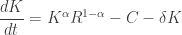
Whereas simple or static optimisation problems may or may not include constraints (conditions a solution must meet), dynamic optimisation problems invariably include constraints in the form of state equations defining the rates of change of state variables. In my problem, the state equation for capital relates growth of capital to income, consumption and depreciation, while that for the resource relates depletion of the stock of resource to use of the resource:

$\dfrac{dK}{dt}=K^{\alpha}R^{1-\alpha}-C-\delta K$

$\dfrac{dS}{dt}= -R$

So far so good. But that’s just setting up the problem. It’s the solving that can be difficult, and is presumably the reason why the topic did not feature in my course syllabus. After all, universities need to recruit students, and those wishing to study environmental economics at graduate level may have taken various first degrees in various disciplines – economics, environmental science, agriculture, etc – not always with a strong mathematical content.

In outline, the method of solution is this. Drawing on the objective function and state equations, you set up an expression known as a Hamiltonian, which will contain one or more additional variables known as costate variables. Using the Hamiltonian, you derive various necessary or first-order conditions that any solution must satisfy. Tests must then be applied to assess whether these necessary conditions are also sufficient. If they are, these conditions will define a unique solution, but further work is then needed to derive, in explicit form, the time paths of the control and other variables.

Why is this difficult? Firstly, it isn’t (to me at least) intuitive. In simple optimisation without constraints, it’s fairly easy to grasp the ideas that the first derivative of a function is its gradient, that the gradient must be zero for a maximum or minimum, and that the second derivative is needed to determine which. But I could not make such a statement about dynamic optimisation. I can apply the maximum principle, but I would not claim to understand, either intuitively or more formally, why it works. Secondly, it isn’t easy to interpret formulae containing costate variables. I know that costate variables in an economic context represent shadow prices, but in a dynamic setting one encounters formulae containing rates of change of shadow prices, which seem one step further removed from ‘real’ economic variables like capital or income. Thirdly, when as is often the case the objective function concerns the discounted present value of some stream of values, care is needed to ensure consistency in using either present (discounted) or current (non-discounted) values, the latter requiring a current-value Hamiltonian and adjustments to the normal conditions, and interpretation of the results accordingly. Fourthly, the necessary conditions relating to the time horizon and values of state variables at that time, known as transversality conditions, need to be carefully considered – not especially difficult, perhaps, but one more issue on top of everything else, and one which can highlight any vagueness in the original formulation of the problem. Fifthly, the tests for sufficiency, such as the Mangasarian and Arrow conditions, involving consideration of whether functions are concave, can be complex to apply: it can be tempting to bypass them and just assume that the necessary conditions are sufficient, but that risks major error if, for example, the optimum is a corner solution.

Finally, when it comes to deriving explicit time paths from the necessary conditions, the devil is in the detail. Rarely is the derivation a matter of elementary algebra. Sometimes it requires solution of differential equations (online solvers such as that in Wolfram Alpha Widgets (5) can be useful, but cannot handle all such equations). Often, especially for problems with multiple state or control variables, there is no exact analytic solution, and approximate numerical methods such as my trial and error with spreadsheets are all that is available.

The issue then for designers of graduate-level courses in environmental economics is this. Omitting the technique of dynamic optimisation is unsatisfactory. But a requirement to be able to solve dynamic optimisation problems unaided would be asking too much of most students, and probably deter applicants. The sensible solution, I suggest, is to require a knowledge of the technique that stops short of an ability to solve dynamic optimisation problems unaided. For example, students might be expected to be able to:

Identify the sort of problems that require the technique, and give examples from environmental and natural resource economics.
Formulate mathematically a dynamic optimisation problem given in words.
Identify the state and control variables in a given problem.
Derive, for simple cases, the Hamiltonian and necessary conditions for a given problem.
Draw inferences from the necessary conditions in cases where this is a matter of simple algebra.
Discuss the complications that can arise in deriving an explicit solution from the necessary conditions.

A more in-depth treatment of dynamic optimisation might also be included in a course as an option, perhaps combined with other techniques such as econometrics under a heading such as ‘quantitative techniques’.

Notes and References

Stranlund J K Lecture 8 Dynamic Opimization http://people.umass.edu/resec712/documents/Lecture8DynamicOptimization.pdf
Perman R, Ma Y, McGilvray J & Common M (3^rd ed’n 2003) Natural Resource and Environmental Economics Pearson Addison Wesley pp 480-505, 512-7, 548-53 & 574-81.
Wikipedia: Pontryagin’s Maximum Principle https://en.wikipedia.org/wiki/Pontryagin%27s_maximum_principle
Buchhholz W, Dasgupta S & Mitra T (2005) Intertemporal Equity and Hartwick’s Rule in an Exhaustible Resource Model Scandinavian Journal of Economics 107(3) pp 547-561 (Modelling of depreciation is introduced on p 551 and the stated result is on p 553 (case $\theta = 1$ and $\delta > 0$ ).
Wolfram Alpha Widgets: General Differential Equation Solver http://www.wolframalpha.com/widgets/view.jsp?id=e602dcdecb1843943960b5197efd3f2a