The literature on the zonal travel cost method (ZTCM) contains occasional suggestions that results can be sensitive to zone definition. My exploratory analysis strongly supports this view.

Originally posted 14/5/2014 as “The Travel Cost Method – Another Pitfall”.  Re-posted following site reorganisation 21/6/2016.

In a previous post, I outlined some well-known pitfalls of the travel cost method. Here I describe and illustrate a pitfall of the zonal version of the method that seems not to be as well-known as it should be.

Introduction

It is generally accepted that research results should be replicable. For a zonal travel cost study, replicability most obviously requires that the same method of analysis applied to data from repeated on-site surveys should lead to similar results. Another requirement, I propose, is that repeated analysis of data from a single on-site survey, aggregated within different zone specifications, should also lead to similar results. I shall refer to this as zonal replicability.

What is the basis for this second requirement? One argument refers to the general scientific maxim, discussed in this post, that repeated tests or measurements should replicate the essential and vary the inessential. Organising points of visitor origin into zones is an essential feature of the zonal travel cost method, but the particular zone specification (often driven by data availability) can hardly be regarded as essential. A more specific argument focusses on the central assumption of the travel cost method, namely, that people would respond to a site entrance fee in the same way that they are found to respond to an equivalent travel cost. This assumption, though it can be challenged, has at least some intuitive plausibility. Suppose however that we were to identify a particular zone specification, and make the assumption that people would respond to a site entrance fee in the same way that they are estimated, using that zone specification, to respond to an equivalent travel cost. An assumption which privileged one particular zone specification in this way would lack plausibility, since it would beg the question whether alternative zone specifications would lead to different findings.

There are many references in the ZTCM literature to the problem of aggregation bias, that is, trip-generating function parameters estimated from aggregate data generally may not accurately reflect individual behaviour (1a-b). It is, perhaps, a short step to the idea that different aggregation structures might yield results that are biased to different degrees or in different directions, but rarely has this step been taken. A notable exception is Bateman (1993), who identified as a feature of ZTCM the possibility of increasing or reducing valuation estimates by respecifying zones (2).

A ZTCM study by Gillespie Economics (2007) includes a statement that consumer surplus estimates were tested for sensitivity to zone specification (3). However, little detail was provided as to the number of alternative zone specifications and how they were chosen. It is unclear therefore how much weight can be placed on the reported finding that differences in consumer surplus estimates were less than 2.5%.

Early applications of ZTCM specified zones consisting of concentric rings. Sutherland (1982) demonstrated that consumer surplus estimates could be sensitive to ring width (4). However, most recent applications of ZTCM use irregular zone specifications, often based on administrative or census districts. My analysis considers the effect on results of alternative irregular zone specifications.

Method

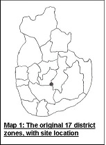
A special case of zonal replicability relates to alternative zone specifications obtained by selective merging of a study’s original zones. If results are found not to be replicable even in such a case, then a fortiori they will not be replicable across the full range of alternative zone specifications. I explored replicability of this kind using data from a study by Rathnayake and Gunawardena (2011) of Horton Plains National Park, Sri Lanka (5), which I chose mainly because unlike many published studies it discloses its full zonal data. This study used data on a sample of visitors, aggregated within 17 of Sri Lanka’s districts together occupying most of the centre and south of the island. Map 1 below shows the 17 district zones, and Chart 1 plots the original zonal data.

My re-analysis of the data followed the original study in treating travel cost as the only independent variable in the trip-generating functions and assuming a linear functional form.  However, to address heteroscedasticity I departed from the original study in estimating the trip-generating functions using weighted least squares, giving higher weightings to zones with larger populations and/or lower visit rates, characteristics which theory suggests will be associated with lower variability in visit rates (7a-b).

To explore zonal replicability, I first obtained a random sample of alternative zone specifications.  The purposes of the sample were: firstly, to support inferences about a wider population of alternative zone specifications without having to make separate calculations for each specification; and secondly, to facilitate illustration of the range of results from alternative zone specifications with examples that cannot plausibly be dismissed as highly unusual or ad hoc constructions.

The sample frame consisted of all possible groupings of the 17 districts into eight zones consisting of seven pairs and one triple, the districts within each pair and triple being required to be adjacent (8).  The number of such groupings was found to be 356.  A sample of 30 zone specifications was then selected by simple random sampling.  Visit rates and travel costs for each merged zone were calculated as population-weighted averages of their values for its constituent districts.  The trip-generating functions for each of the 30 zone specifications were then estimated, and from these the demand curves and consumer surpluses were obtained in the standard way (9).

From the distributions of the estimates of the trip-generating function coefficients and consumer surplus over the sample of 30 zone specifications, inferences were drawn about their distributions over the population of 356 zone specifications.

 Results

A convenient unit-free measure of the variability of a distribution is its coefficient of variation, the ratio of its standard deviation to its mean.  Table 1 shows the estimated coefficients of variation of the distributions of the trip-generating function coefficients over the population of 356 zone specifications.  The variability measured here is due solely to different zone specifications applied to the same underlying data. It is quite distinct from the imprecision of individual coefficient estimates arising from the underlying data being sample-based.

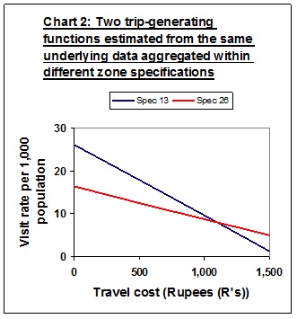
The two coefficients are negatively correlated, a higher constant being associated with a more negative travel cost coefficient, and  the estimated trip-generating functions intersect in the region where most of the original data points are concentrated.  Chart 2 shows the trip-generating functions with the highest and lowest constants among the sample, illustrating the range of variability and the intersection property, and Maps 2 and 3 show the relevant zone specifications.

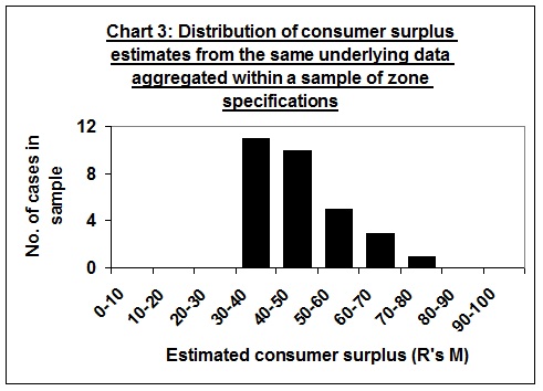
Chart 3 shows the distribution of consumer surplus estimates within the sample.  The coefficient of variation is 0.222, larger than for either of the trip-generating coefficients. The highly skewed distribution suggests that the distribution of consumer surplus estimates over the population of 356 zone specifications may be far from normal, and there was therefore no simple way to estimate the coefficient of variation of that distribution.  Nevertheless, the range of estimates over the population must be at least as large as that over the sample, which is from R’s 36.4 M (Specification 13) to R’s 76.7 M (Specification 26), a factor of 2.1.

Discussion

The finding that different zone specifications can lead to different results is an example of a general problem in spatial modelling, known to geographers and statisticians as the modifiable areal unit problem.  In general terms, the problem is that spatial data can be aggregated in many different ways which can lead to different results on analysis of the aggregate data.  A useful source is Openshaw (10).  A rare reference to the problem in the literature on the travel cost method is by Brainard, Lovett & Bateman 1997, who characterise that literature, with some justice, as spatially naïve (11).

The finding that the variability over different zone specifications of the consumer surplus estimates can be greater than that of the trip-generating function coefficients parallels a similar finding by Adamowicz, Fletcher & Graham-Tomasi (1989) in respect of variability arising from sampling error (12).  An underlying reason in both cases is that, even if the trip-generating function is linear, there is non-linearity in the calculation of the consumer surplus from the trip-generating function.

It was not an aim of this analysis to test the replicability of the results of the original study by Rathnayake & Gunawardena.  A comparison of the results from alternative specifications of 8 zones with those from the original specification of 17 zones would conflate two issues: the effect of alternative specifications of a given number of zones, and the effect of varying the number and size of zones.  That specifications with more and smaller zones will tend to exhibit less variability in their results than those with fewer and larger zones is an interesting and plausible hypothesis, but not one that has been explored here.  The most direct relevance of this analysis is to ZTCM studies where the original zone specification consists of about 8 zones.

Examples of such zone specifications that have been used in ZTCM studies include South African provinces (9 zones), Ugandan districts (10 zones), groups of Indian states (10 zones), groups of Chinese provinces (9 zones), and (for a site attracting many international visitors) a specification based largely on continents (7 zones) (13a-e).  Given the finding that alternative specifications of 8 zones around the Sri Lankan site can lead to results differing by a factor of more than 2, it seems likely that results based on specifications of 7-10 zones in other parts of the world would be found to vary markedly with the particular specification chosen, holding the number of zones constant.  If so, results based on one particular specification are fairly likely to be markedly biased (since if different specifications lead to a wide range of results, only a small proportion can lead to results that approximate closely to the true result).  Moreover, if the result of a ZTCM study based on about 8 zones is presented simply as a point estimate of consumer surplus, then it is likely to lack zonal replicability.

Should it be inferred that ZTCM is so unreliable that it should be abandoned?  That would be too sweeping a conclusion I suggest.  All methods for valuing non-market environmental goods have their limitations, and we need ZTCM among our menu of available methods, especially for circumstances in which aggregate data is all we can collect at reasonable cost.  What certainly should be inferred is that the results of ZTCM studies should be presented in a way which clearly communicates their possible inaccuracy.  This requires explicit reference both to sampling error arising from the underlying data being sample-based and possible bias arising from the choice of zone specification to aggregate that data.  A useful topic for further research would be to test the hypothesis that variability in results can be reduced by specifying smaller zones, with a view to developing guidance on zone size.

Supporting Analysis

I can provide the supporting analysis on request (in MS Excel 2010 format).  My email address is in About.

Notes & References

1a. Rosenthal D H & Anderson J C (1984)  Travel Cost Models, Heteroskedasticity, and Sampling  Western Journal of Agricultural Economics 9(1) p 58-60;   http://ageconsearch.umn.edu/bitstream/32368/1/09010058.pdf

1b. Hellerstein D (1995) Welfare Estimation Using Aggregate and Individual-Observation Models: A Comparison Using Monte Carlo Techniques  American Journal of Agricultural Economics 77 (August 1995) p 623

2.  Bateman I J (1993)  Valuation of the environment, methods and techniques: revealed preference methods, in Turner R K (ed) Sustainable Environmental Economics and Management: Principles and Practice  Belhaven Press, London p 230

3.  Gillespie Economics (2007) The Recreation Use Value of NSW Marine Parks (Report for the New South Wales Department of Environment and Climate Change) p 4  http://www.environment.nsw.gov.au/resources/research/RecreationUseValueNSWMarineParks.pdf

4. Sutherland R J (1982)  The Sensitivity of Travel Cost Estimates of Recreation Demand to the Functional Form and Definition of Origin Zones  Western Journal of Agricultural Economics  July 1982 pp 95-7 http://ageconsearch.umn.edu/bitstream/32416/1/07010087.pdf

5.  Rathnayake R M W & Gunawardena U A D P (2011)  Estimation of Recreational Value of Horton Plains National Park in Sri Lanka: A Decision Making Strategy for Natural Resources Management  Journal of Tropical Forestry and Environment 1(1) pp 71-86  http://journals.sjp.ac.lk/index.php/JTFE/article/view/86

6. Rathnayake & Gunawardena, as 5 above, pp 79-80

7a. Bowes M D & Loomis J B (1980) A Note on the Use of Travel Cost Models with Unequal Zonal Populations  Land Economics 56(4) p 468

7b. Christensen J B & Price C (1982) A Note on the Use of Travel Cost Models with Unequal Zonal Populations: Comment  Land Economics 58(3) pp 396 & 399

8.  Identifying all such groupings was a challenging mathematical problem, solved by a method involving representation of each district by a distinct prime integer, and each pair and triple by the product of the primes representing its constituent districts.  The use of products of distinct primes ensures that zones are non-overlapping if and only if their products have no common factor greater than one.  In this way the spatial problem was transformed into an arithmetical problem which could be solved in a spreadsheet.

9.  See for example Perman R, Ma Y, McGilvray J & Common M (3^rd ed’n 2003) Natural Resource & Environmental Economics   Pearson / Addison Wesley, Harlow, England  pp 413-4

10. Openshaw S (1984) The Modifiable Areal Unit Problem  Geo Books, Norwich, England   http://qmrg.org.uk/files/2008/11/38-maup-openshaw.pdf

11. Brainard J S, Lovett A A & Bateman I J (1997)  Using isochrone surfaces in travel-cost models  Journal of Transport Geography  5(2)p 118

12. Adamowicz W L, Fletcher J J & Graham-Tomasi T (1989) Functional Form and the Statistical Properties of Welfare Measures  American Journal of Agricultural Economics 71 pp 416 & 418

13a. Turpie J & Joubert A (2004)  The value of flower tourism on the Bokkeveld Plateau – a botanical hotspot  Development Southern Africa  21(4) pp 647 & 650

13b. Buyinza M, Bukenya M & Nabalegwa M (2007) Economic Valuation of Bujagali Falls Recreational Park, Uganda  Journal of Park and Recreation Administration 25(2) p 21  http://js.sagamorepub.com/jpra/article/view/1362

13c. De U K & Devi A (2011) Valuing Recreational and Conservation Benefits of a Natural Tourist Site: Case of Cherrapunjee  Journal of Quantitative Economics 9(2) p 162

13d. Liu Y, Nie L & Liao B (2012)  The Recreational Value of Bama in China: One of the Five World’s Longevity Townships  Business and Management Research 1(4) p 149  http://www.sciedu.ca/journal/index.php/bmr/article/view/2104

13e. Mugambi M D & Mburu J I (2013)  Estimation of the Tourism Benefits of Kakamega Forest, Kenya: A Travel Cost Approach  Environment and Natural Resources Research 3(1) p 65  http://www.ccsenet.org/journal/index.php/enrr/article/view/20073