Dynamic Optimisation: A Fully Worked Example

In a previous post, I referred to the importance in environmental and natural resource economics of the technique of dynamic optimisation, also known as optimal control. However, the technique is difficult, and worked examples in textbooks or on the web often seem to pass over key points. Here I present my own example, which I describe as fully worked because it shows every step from the largely verbal statement of the problem to the optimal paths of the key variables and the maximum value of the objective functional, identifying some options and pitfalls along the way. It is intended for readers familiar with elementary algebra, calculus and static optimisation who have at least begun to study dynamic optimisation.

The Problem

Capital $K,$ is the only factor of production and is not subject to depreciation. The initial capital stock is $100,$ . Output is at a rate $0.5K,$ , and may be used as consumption $C,$ or investment $I,$ , the latter being added to $K,$ . The instantaneous utility function $U_t$ is $\ln(C_t)$ . We are required to maximise social welfare $W,$ from time $t = 0,$ to $10,$ , where social welfare is defined as the integral of instantaneous utility subject to a continuous discount factor of $10\%,$ per time period.

A Note on Notation

A widely used convention is that the subscript $t,$ , as in $C_t$ , indicates discrete time, and that a variable in continuous time should be written as in $C(t),$ . I find however that it saves a little keying time, and results in less cluttered formulae, to use the subscript approach for continuous time, and sometimes to omit the $t,$ altogether when it is clear from the context. More conventionally, I use the notation $\dot C,$ to indicate a time-derivative, and $\ddot C,$ for a second time-derivative.

I use Latex to display mathematical symbols and formulae. However, using Latex within a WordPress blog is not entirely straightforward, one problem being to obtain a satisfactory vertical alignment of symbols within text paragraphs. The commas which follow some symbols are a workaround which corrects vertical alignment in many (though not all) cases and seem to me preferable to the alternative of displaying symbols – like $K$ for example – with their base lower than that of the surrounding text.

Writing the Problem in Mathematical Formulae

Our problem statement above contains the symbols $K, C, I, U, W, t$ . The first question we should consider is whether we need all these for a precise mathematical formulation. It is clear that we can dispense with $U,$ and relate $W,$ directly to $C,$ , writing the objective functional as:

$\textrm{Maximise }W=\int_0^{10}(\ln(C_t))e^{-0.1t}dt\qquad(1)$

We need $K,$ which is clearly the state variable, but what is the control variable? Since $C + I = 0.5K,$ , either of $C,$ or $I,$ determines the other. Nothing in the problem statement indicates that one is a choice variable and the other a residual. Either could be the control variable, but we do have to choose (because the method requires maximisation of the Hamiltonian or Lagrangian with respect to the control variable). Let us choose $C,$ as the control variable (but Alternative 1 below will show that choosing $I,$ leads to the same results). We therefore write the equation of motion as:

$\dot K=0.5K-C\qquad(2)$

We also have the boundary conditions:

$K_0=100\ \textrm{and }K_{10}\ \textrm{free}\qquad(3)$

Does that complete the formulation of the problem? No!

Pitfall 1

If we rely on the formulation above, there is nothing to prevent negative consumption, with investment $\dot K,$ exceeding output and $W,$ undefined (because the log of a negative quantity is undefined). There is also nothing to prevent negative investment. Thus the above formulation allows a time path in which capital is initially accumulated, but towards the end of the time period is run down to zero, enabling consumption to exceed output. That could be a desirable scenario if the capital is in the form of a good which can also be consumed. More typically, however, capital cannot be consumed and therefore consumption cannot exceed output, and the above formulation will therefore lead to erroneous results by permitting more consumption than is feasible. Indeed, there is nothing in the formulation to rule out the combination of infinite consumption and infinite negative investment.

We therefore add two constraints and, to prepare for writing the required Lagrangian function, rewrite each as a quantity to be less than or equal to a constant, in these cases zero:

$C_t \geq 0\ \forall t \in [0,10]\ \textrm{and so } -C_t \leq 0\qquad(4)$

$C_t \leq 0.5K_t\ \forall t \in [0,10]\ \textrm{and so } C_t-0.5K_t \leq0\qquad(5)$

Although we also require that capital should not be negative, we need not specify this as a further constraint since it is is implied by the combination of $K_0=100$ and $\dot K\geq 0,$ , the latter following from the equation of motion together with constraint (5). Indeed, these imply the stronger condition $K_{10} \geq 100$ . The combination of (1) to (5) completes the mathematical formulation of the problem.

The Value of W for Two Naïve Solutions

Before applying the method of optimal control, let us consider a couple of simple and feasible time paths for consumption and calculate the implied values of $W,$ . The results will provide a benchmark against which we can compare our final result. Suppose first that there is no investment and all output is consumed. Then capital is always $100,$ and consumption is always $0.5(100) = 50,$ . Hence:

$W=\int_0^{10}(\ln50)e^{-0.1t}dt$

$W=3.912\left[-10e^{-0.1t}\right]_0^{10}=3.912(-10e^{-1}+10)=\mathbf{24.73}$

Now suppose that output is always divided equally between consumption and investment. Before we can calculate $W,$ we need to find the time path of capital by solving the differential equation:

$\dot K =0.5(0.5K)=0.25K\qquad(6)$

Making the standard substitution $K, = e^{bt}$ so that $\dot K,= be^{bt}$ we have:

$be^{bt}=0.25e^{bt}\ \textrm{and so } b=0.25\qquad(7)$

Hence for some constant $c,$ :

$K_t=ce^{0.25t}\qquad(8)$

Since $K_0 = 100$ we can infer that $c=100,$ and so:

$K_t=100e^{0.25t}\ \textrm{and so } C_t=0.5(0.5K_t)=25e^{0.25t}\qquad(9)$

Hence:

$W=\int_0^{10}(\ln(25e^{0.25t})e^{-0.1t}dt=\int_0^{10}(3.219+0.25t)e^{-0.1t}dt\qquad(10)$

$W=\left[-(32.19+2.5t+25)e^{-0.1t}\right]_0^{10}$

$W=-82.19e^{-1}+57.19=\mathbf{26.95}$

As we might expect, allocating half of output to investment, allowing capital to accumulate and increase output as time goes on, yields a higher $W,$ than simply consuming all output. But there is no reason to expect that this value of $W,$ is the maximum.

Necessary Conditions for a Solution

From (1) and (2) we obtain the Hamiltonian, introducing a costate variable $\lambda_t$ :

$H=(\ln C)e^{-0.1t}+\lambda (0.5K-C)\qquad(11)$

This is a present value Hamiltonian because it retains the discount factor in the objective functional and so converts $\ln C_t$ at any time to its present value, that is, its value at time $0,$ . An alternative approach will be considered below. Because we have two inequality constraints, we must extend the Hamiltonian to form a Lagrangian, introducing two Lagrange multipliers $\mu_t$ and $\nu_t$ :

$\mathcal{L}=(\ln C)e^{-0.1t}+\lambda (0.5K-C)+\mu C+\nu (0.5K-C)\;(12)$

The expressions in brackets after the Lagrange multipliers are from the inequality constraints (4) and (5) with signs changed. The general rule here is that given a constraint $g, \leq k$ and writing $\theta_t$ for the associated multiplier, the term to be included in the Lagrangian is $\theta_t(k-g)$ .

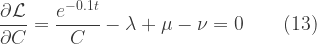
Applying the maximum principle, we have to maximise the Lagrangian with respect to the control variable $C_t$ at all times. In this case, the Lagrangian is differentiable with respect to $C_t$ , so we can try to use calculus to find a maximum. But we also need to consider whether there might be a corner solution, that is, a solution at either of the limits of the constrained range of $C,$ , which are $0,$ and $0.5K,$ . We can rule out the possibility of a maximum at $t = 0,$ , since $\ln 0,$ equals minus infinity. But there is no obvious reason why there should not be a maximum at $C, = 0.5K$ for at least some values of $t,$ , so we should keep this possibility in mind. Setting the derivative with respect to $C,$ of the Lagrangian equal to zero we have:

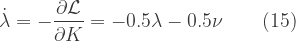
$\dfrac{\partial \mathcal{L}}{\partial C}=\dfrac{e^{-0.1t}}{C}-\lambda+\mu-\nu=0\qquad(13)$

The maximum principle also requires the conditions:

$\dot K=\dfrac{\partial \mathcal{L}}{\partial \lambda}=0.5K-C\qquad(14)$

$\dot {\lambda}=-\dfrac{\partial \mathcal{L}}{\partial K}=-0.5\lambda-0.5\nu\qquad(15)$

Although the effect of (14) is merely to repeat the equation of motion (2) it is standard practice to write it out at this point in the working. We also require the Kuhn-Tucker conditions in respect of the two inequality constraints, conditions (17) being known as the complementary slackness conditions.

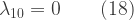
$\mu \geq 0\ \textrm{and } \nu \geq 0\ \forall t \in [0,10]\qquad(16)$

$\mu C=0\ \textrm{and }\nu (0.5K-C)=0\ \forall t \in [0,10]\qquad(17)$

Finally, there is the transversality condition. With a fixed terminal time, but terminal capital free subject to the implied condition $K_{10} \geq 100$ , we have the situation known as a truncated vertical terminal line. Therefore we provisionally adopt the condition:

$\lambda_{10}=0\qquad(18)$

However, we will have to check that the resulting solution is consistent with the condition $K_{10} \geq 100$ (and if not we must recalculate the solution with $K_{10}$ fixed at $100,$ ). (12) to (18), with the provisos noted, constitute the necessary conditions for a maximum.

Sufficiency of the Necessary Conditions

We will test whether the Mangasarian conditions are satisfied. The basic conditions are:

(A) The integrand of the objective function, $(\ln C)e^{-0.1t},$ , must be differentiable and concave in the control and state variables, $C,$ and $K,$ , jointly.

(B) The equation of motion formula, $0.5K-C,$ , must be differentiable and concave in $C,$ and $K,$ jointly.

(C) If the equation of motion formula, $0.5K-C,$ , is non-linear in either $C,$ or $K,$ , then in the optimal solution we must have $\lambda_t \geq 0$ for all $t,$ .

Considering these in turn:

Condition (A) is satisfied since, applying a calculus test for concavity:

$\dfrac{\partial((\ln C)e^{-0.1t})}{\partial C}=\dfrac{e^{-0.1t}}{C}\ \textrm{ so }\dfrac{\partial^2((\ln C)e^{-0.1t})}{\partial C^2}=-\dfrac{e^{-0.1t}}{C^2} \leq 0\ \forall t\quad(19)$

We need not consider $K,$ here since it does not occur in the integrand.

Condition (B) is satisfied since the formula $0.5K-C,$ is linear in both $C,$ and $K,$ and therefore concave, linearity being sufficient for concavity (there is no requirement for strict concavity).

Condition (C) is satisfied since, again, the formula $0.5K-C,$ is linear in both $C,$ and $K,$ .

For our problem, a further condition is needed for each of the inequality constraints, the general rule being that if a constraint is represented in the Lagrangian by the expression $\theta (k-g)$ where $k,$ is a constant, the required condition is that $g,$ be jointly convex in the control and state variables:

(D) $-C,$ must be convex in $C,$ and $K,$ jointly.

(E) $C-0.5K,$ must be convex in $C,$ and $K,$ jointly.

These conditions are satisfied since the functions are linear (again there is no requirement for strict convexity).

Thus the Mangasarian conditions are satisfied, so we can conclude that the necessary conditions (12) to (18) are also sufficient for a maximum (and need not consider the more complex Arrow conditions).

Inferences from the Necessary Conditions

Using a common approach to simplification, we differentiate (13) with respect to time and then use (15) to substitute for $\dot{\lambda},$ :

$\dfrac{-0.1e^{-0.1t}C-\dot Ce^{-0.1t}}{C^2}-\dot{\lambda}+\dot{\mu}-\dot{\nu}=0\qquad(20)$

$\dfrac{-0.1e^{-0.1t}C-\dot Ce^{-0.1t}}{C^2}+0.5\lambda+0.5\nu+\dot{\mu}-\dot{\nu}=0\qquad(21)$

Using (13) again we can eliminate $\lambda,$ and $\nu,$ (but not $\dot{\nu},$ ):

$\dfrac{-0.1e^{-0.1t}C-\dot C e^{-0.1t}}{C^2}+\dfrac{0.5e^{-0.1t}}{C}+0.5\mu+\dot{\mu}-\dot{\nu}=0\qquad(22)$

$-0.1e^{-0.1t}C-\dot Ce^{-0.1t}+0.5e^{-0.1t}C+(0.5\mu+\dot{\mu}-\dot{\nu})C^2=0\,(23)$

Collecting the terms in $C,$ and using the complementary slackness condition (17) $\;\mu C=0,$ (which, since $C,$ can never be zero as $\ln 0,$ equals minus infinity, implies $\mu =0,$ and therefore $\dot{\mu}= 0,$ for all $t,$ ):

$0.4e^{-0.1t}C-\dot Ce^{-0.1t}-\dot{\nu}C^2=0\qquad(24)$

Using the equation of motion (2) to substitute for $C,$ :

$0.4e^{-0.1t}(0.5K-\dot K)-(0.5\dot K-\ddot K)e^{-0.1t}-\dot{\nu}(0.5K-\dot K)^2)=0\quad(25)$

Collecting terms in $e^{-0.1t},$ we have the differential equation:

$e^{-0.1t}(\ddot K-0.9\dot K+0.2K)-\dot{\nu}((0.5K)^2-K\dot K+(\dot K)^2=0\qquad(26)$

Before proceeding we will explore two alternative approaches.

Alternative 1: Investment as the Control Variable

Suppose we take investment $I,$ rather than consumption $C,$ to be the control variable. The utility function is still $\ln C,$ which we will now have to write as $\ln(0.5K-I),$ , so the objective functional will be:

$\textrm{Maximise }W=\int_0^{10}(\ln(0.5K-I))e^{-0.1t}dt\qquad(A1)$

The equation of motion will be simply:

$\dot K=I \qquad(A2)$

This is not tautologous since it implies that investment is the only cause of change in capital, eg there is no depreciation. The inequality constraints become:

$I-0.5K\leq 0\;\; \textrm{and }\;-I\leq 0\qquad(A3)$

Hence the Lagrangian is:

$\mathcal{L}=(\ln(0.5K-I))e^{-0.1t}+\lambda I+ \mu (0.5K-I)+\nu I\qquad(A4)$

From the Lagrangian we derive the conditions:

$\dfrac{\partial\mathcal{L}}{\partial I}=\dfrac{-e^{-0.1t}}{0.5K-I}+\lambda -\mu +\nu=0\qquad(A5)$

$\dot K=\dfrac{\partial\mathcal{L}}{\partial\lambda}=I\qquad(A6)$

$\dot {\lambda}=-\dfrac{\partial\mathcal{L}}{\partial K}=\dfrac{-0.5e^{-0.1t}}{0.5K-I}-0.5\mu\qquad(A7)$

We also have the complementary slackness conditions:

$\mu(0.5K-I)=0\;\;\textrm{and }\nu I=0\qquad(A8)$

Differentiating (A5) with respect to time, using (A7) to substitute for $\dot{\lambda},$ , and substituting $\dot K,$ for $I,$ :

$\dfrac{0.1e^{-0.1t}(0.5K-\dot K)+(0.5\dot K-\ddot K)e^{-0.1t}}{0.5K-\dot K)^2}-\dfrac{0.5e^{-0.1t}}{0.5K-\dot K)}-0.5\mu -\dot{\mu}+\dot{\nu}=0\quad(A9)$

$e^{-0.1t}(-\ddot K+0.4\dot K+0.05K)-0.5e^{-0.1t}(0.5K-\dot K)+(-0.5\mu - \dot{\mu}+\dot{\nu})(0.5K-\dot K)^2=0\quad(A10)$

Collecting terms in $e^{-0.1t},$ and using the first complementary slackness condition to eliminate $\mu ,$ and $\dot{\mu},$ we have:

$e^{-0.1t}(-\ddot K+0.9\dot K-0.2K)+\dot{\nu}((0.5K)^2-K\dot K+\dot K^2)=0\quad(A11)$

It can be seen that this is equation (26) above with signs reversed, so thereafter we can proceed as in the main line of reasoning.

Alternative 2: the Current Value Hamiltonian

When the objective functional contains a discount factor, an alternative method is to use the current value Hamiltonian. Where there are inequality constraints, this leads to a current value Lagrangian, which for our problem can be written:

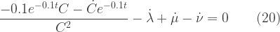
$\mathcal{L}_C=\ln C+\rho (0.5K-C)+\sigma C+ \tau (0.5K-C)\qquad(A12)$

where the multipliers $\rho ,\sigma ,\tau$ are equal respectively to the original multipliers $\lambda ,\mu ,\nu$ each multiplied by $e^{-0.1t},$ . In the necessary conditions, the equivalent of (13) is slightly simplified by the absence of the discount factor:

$\dfrac{\partial\mathcal{L}_C}{\partial C}=\dfrac{1}{C}-\rho +\sigma -\tau =0\qquad(A13)$

On the other hand the equivalent of (15) requires an extra term $0.1\rho ,$ (the discount rate being $0.1,$ ):

$\dot{\rho}=-\dfrac{\partial\mathcal{L}_C}{\partial K}+0.1\rho =-0.5\rho-0.5\tau+ 0.1\rho =-0.4\rho-0.5\tau\qquad(A14)$

The difference between the coefficients in the terms $0.5\lambda ,$ in (15) and $0.4\rho ,$ in (A14) may seem trivial, but it leads to additional complexity later in the reasoning. The equivalent of (24), which I re-write here for ease of reference:

$0.4e^{-0.1t}C-\dot Ce^{-0.1t}-\dot{\nu}C^2=0$

is found to be:

$0.4e^{-0.1t}C-\dot Ce^{-0.1t}-(\dot{\rho}-0.1\rho )C^2=0\ \quad(A15)$

The more complex coefficient of $C^2,$ in turn makes it slightly more complicated to solve what below I call Case 2. This is not to argue against the current value approach, still less to suggest that it represents a pitfall. But whether on balance it simplifies matters, as is often suggested, seems to depend on the type of problem.

Solving the Differential Equation

Our differential equation (26) looks rather intractable, but we can simplify matters by considering separately the two cases $\nu = 0,$ and $\nu \neq 0$ . To be more precise, we consider:

Case 1: $\nu = 0,$ over some time interval.

Case 2: $\nu \neq 0$ over some time interval.

Since Case 1 implies that $\nu ,$ is constant over the relevant interval, we can infer that $\dot{\nu}= 0,$ over that period. Equation (26) therefore simplifies to:

$\ddot K-0.9\dot K+0.2K=0\qquad(27)$

The standard method for this type of differential equation is to make the substitution $K=e^{xt},$ implying $\dot K=xe^{xt},$ and $\ddot K=x^2e^{xt},$ . After dividing through by $e^{xt},$ we are left with the equation:

$x^2-0.9x+0.2=0\qquad(28)$

By factorisation or by the quadratic equation formula, this is neatly solved by $x=0.4, \textrm{ or }0.5$ . Hence the solution to the differential equation (27) is:

$K=c_1e^{0.4t}+c_2e^{0.5t}\qquad(29)$

where $c_1,c_2$ are constants to be found (generally a second order differential equation requires two constants of integration). Differentiating (29) with respect to time we can infer:

$\dot K=0.4c_1e^{0.4t}+0.5c_2e^{0.5t}\qquad(30)$

$C=0.5K-\dot K=0.1c_1e^{0.4t}\qquad(31)$

Pitfall 2

Having obtained equations (29) to (31) it is tempting to think that our work is almost complete. Putting $t=0,$ in (29) we have:

$100=c_1+c_2\qquad(P1)$

Since investment right at the end of the time period can do nothing to increase consumption within the time period, we can infer that $\dot K=0,$ at $t=10,$ . Hence, putting $t=10,$ in (30):

$0=0.4c_1e^4+0.5c_2e^5\qquad(P2)$

$-0.4c_1=0.5e(100-c_1) \quad(P3)$

$c_1(0.5e-0.4)=50e\qquad(P4)$

$c_1=\dfrac{50e}{0.5e-0.4}=141.7 \textrm{ and }c_2=100-c_1=-41.7\quad(P5)$

Substituting into (31):

$C=14.17e^{0.4t}\qquad(P6)$

Therefore:

$W=\int_0^{10}(\ln (14.17e^{0.4t})e^{-0.1t}dt=\int_0^{10}(2.651+0.4t)e^{-0.1t}dt\quad(P7)$

$W=\left[-(26.51+0.4t+40)e^{-0.1t}\right]_0^{10}=-70.51e^{-1}+66.51=\mathbf{27.33}$

As expected, this yields a higher value of $W,$ than either of the naïve solutions considered above. Nevertheless, this is not the time path that maximises $W,$ . The fallacy here is the assumption that our Case 1 applies to the whole period $t=[0,10]$ . Just because $\dot K=0,$ at $t=10,$ , it does not follow that $\dot K\neq 0,$ at all $t<10,$ .

We must also consider Case 2, $\nu \neq 0,$ . Using the second complementary slackness relation (17), this implies that:

$0.5K-C=0\qquad(32)$

Thus Case 2 is what we described above as a corner solution. Using the equation of motion (2) this implies that, within the relevant time range, $\dot K= 0,$ and therefore $\ddot K=0,$ . Hence the differential equation (26) reduces to:

$e^{-0.1t}(0.2K)-\dot{\nu}(0.5K)^2=0\qquad(33)$

$0.2e^{-0.1t}-0.25K\dot{\nu}=0\qquad(34)$

$\dot{\nu}=\dfrac{0.8e^{-0.1t}}{K}\qquad(35)$

Integrating with respect to $t,$ , noting that $K,$ can be treated as a constant since $\dot K= 0,$ :

$\nu =-\dfrac{8e^{-0.1t}}{K}+c_3\qquad(36)$

Which Case is Terminal?

We will now show that, as time approaches $t=10,$ , the system must be in Case 2, with $K,$ constant. This is what we would expect from economic reasoning, since there must be a time beyond which the effect of further investment in making possible higher output and consumption in the remainder of the time period is too small to compensate for the consumption that would be forgone in making that investment. To show this using the method of optimal control, we start from the transversality condition (18), $\lambda_{10}= 0$ . We can therefore reduce (13) at $t=10,$ to:

$\dfrac{e^{-1}}{C_{10}}+ \mu_{10}-\nu_{10}= 0\qquad(37)$

Given the first complementary slackness relation (17), $\mu C,$ , this further simplifies to:

$\dfrac{e^{-1}}{C_{10}}-\nu_{10}= 0\qquad(38)$

This implies that $\nu_{10}\neq 0$ (otherwise $C_{10}$ would be infinite which is impossible given the problem data). So the system cannot be in Case 1 at $t=10$ , and must be in Case 2.

When Does the System Switch from Case 1 to Case 2?

Taking our Case 2 equation (36) at $t=10,$ , and using (38) to substitute for $\nu_{10}$ :

$\dfrac{e^{-1}}{C_{10}}=-\dfrac{8e^{-1}}{K_{10}}+c_3\qquad(39)$

From the equation of motion (2), and since $\dot K=0,$ in Case 2, we can substitute $2C_{10}$ for $K_{10}$ :

$\dfrac{e^{-1}}{C_{10}}=-\dfrac{8e^{-1}}{2C_{10}}+c_3\qquad(40)$

$c_3=\dfrac{e^{-1}}{C_{10}}+\dfrac{4e^{-1}}{C_{10}}=\dfrac{5e^{-1}}{C_{10}}\qquad(41)$

Substituting for $c_3$ in (36):

$\nu =-\dfrac{8e^{-0.1t}}{K}+\dfrac{5e^{-1}}{C_{10}}\qquad(42)$

While the system is in Case 2, $K,$ is constant, so we can replace it by $K_{10}$ and therefore by $2C_{10}$ :

$\nu =-\dfrac{8e^{-0.1t}}{2C_{10}}+\dfrac{5e^{-1}}{C_{10}}=\dfrac{5e^{-1}-4e^{-0.1t}}{C_{10}}\qquad(43)$

Since Case 2, by definition, has $\nu \neq 0,$ , and since from (38) $\nu_{10}>0$ , the system will be in Case 2 while:

$5e^{-1}-4e^{-0.1t}>0\qquad(44)$

$1.25>e^{1-0.1t}\qquad(45)$

$1-0.1t<\ln 1.25=0.223\qquad(46)$

$t>7.77\qquad(47)$

So we can infer that the system is in Case 1 during $t=[0,\;7.77]$ and in Case 2 during $t=(7.77,\;10]$ .

Solving Case 1

Having found the time period over which Case 1 applies, we can now determine the constants $c_1,c_2$ in equations (29) to (31). Taking (29) at $t=0,$ we have:

$100=c_1+c_2\qquad(48)$

Since the system switches to Case 2 at $t=7.77,$ with $\dot K=0,$ , from (30) we have:

$0=0.4c_1e^{0.4(7.77)}+0.5c_2e^{0.5(7.77)}\qquad(49)$

$0=0.4c_1+0.5c_2e^{0.777}\qquad(50)$

$\dfrac{c_2}{c_1}=-0.8e^{-0.777}=\dfrac{100-c_1}{c_1}\qquad(51)$

$-c_1(0.8e^{-0.777}-1)=100\qquad(52)$

$c_1=-\dfrac{100}{0.8e^{-0.777}-1}=158.2\qquad(53)$

$c_2=100-158.2=-58.2\qquad(54)$

Substituting into (29 to (31), we have the time paths of the key variables over $t = [0, 7.77]$ :

$K=158.2e^{0.4t}-58.2e^{0.5t}\qquad(55)$

$\dot K=63.3e^{0.4t}-29.1e^{0.5t}\qquad(56)$

$C=15.8e^{0.4t}\qquad(57)$

Although not essential to solve the problem, it may be of interest to note the time paths, over the same period, of the various multipliers. From the first complementary slackness relation (17) and because $C,$ can never be zero, we can infer that $\mu = ,0$ , and from the definition of Case 1 we have $\nu =0,$ . Substituting these values into (13):

$\dfrac{e^{-0.1t}}{C_t}-\lambda_t=0\qquad(58)$

$\lambda_t=\dfrac{e^{-0.1t}}{15.8e^{0.4t}}=0.0633e^{-0.5t}\qquad(59)$

The value of $\lambda ,$ can be interpreted as the shadow price of the state variable, capital, that is, the amount by which $W,$ could be increased if an extra unit of capital were available at time $t,$ . It can be seen that this value at $t=0,$ is $0.0633,$ , which may seem surprisingly small given the extra consumption over the whole period which an extra unit of initial capital would make possible, but can be shown to be correct given that $W,$ depends on the log of consumption.

Solving Case 2

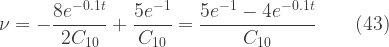
A feature of Case 2 is that $K,$ remains constant. To find at what level it remains constant, we have simply to find its level at $t=7.77,$ , when Case 1 switches to Case 2. Substituting into (55):

$K=158.2e^{0.4(7.77)}-58.2e^{0.5(7.77)}=3540-2832=708\qquad(60)$

This is the value of $K,$ over the period $(7.77,\;10]$ , and enables us to confirm that $K_{10}\geq 100$ and therefore to accept the condition (18), $\lambda_{10}=0$ , without qualification. Over the same period, $\dot K=0,$ and:

$C=0.5(708)=354\qquad(61)$

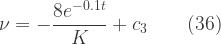
Turning to the multipliers, $\mu =0,$ for the same reason as during Case 1. Substituting for $C,$ in (43):

$\nu =\dfrac{5e^{-1}-4e^{-0.1t}}{354}=0.0052-0.0113e^{-0.1t}\qquad(62)$

Thus $\nu ,$ increases gradually from $0,$ at $t=7.77,$ to $0.0010,$ at $t=10,$ . The positive values of $\nu ,$ when $t>7.77,$ indicate that if the constraint $C_t\leq 0.5K_t$ were relaxed then $W,$ could be increased.

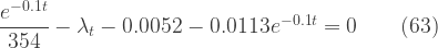
To obtain $\lambda .$ over the same period, we use (61) and (62) to substitute for $C,$ and $\nu ,$ respectively in (13):

$\dfrac{e^{-0.1t}}{354}-\lambda_t-0.0052-0.0113e^{-0.1t}=0\qquad(63)$

$\lambda_t=-0.0052+0.0141e^{-0.1t}\qquad(64)$

Thus $\lambda ,$ falls from $0.0013,$ at $t=7.77,$ to, as expected, $0,$ at $t=10,$ , at which point an extra unit of capital would have no effect within the time period on $C,$ or $W,$ .

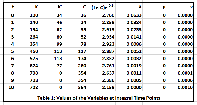
Table 1 below shows the values of all the variables at integral time points over the whole period $[0,\;10]$ , convering Cases 1 and 2.

The Optimal Value of W

It remains to check that the optimal paths we have now identified do indeed result in a larger $W,$ than our best so far – the $27.33,$ obtained from our Pitfall 2. Summing the relevant integrals over the Case 1 and Case 2 periods we have: