Economic Droplets

Fishing and Economic Welfare

Posted on June 21, 2016 by Adam Bailey

Within a static model of a fishery one can identify levels of fishing effort for maximum yield, maximum profits and maximum welfare. Where demand is downward-sloping, effort for maximum welfare will normally be above that for maximum profits but below that for maximum yield.

Originally posted 14/6/2014. Re-posted following site reorganisation 21/6/2016.

In a previous post discussing the reform of the EU’s Common Fisheries Policy, I outlined a model of a fishery in steady state with price flexibility. Here I present that model in mathematical form.

Bioeconomic models of fisheries often take the price of fish as given. This could be for the good reason that a model is intended to represent a local fishery whose output is too small to affect the market price of fish. In the context of textbooks on natural resource economics, there may also be a pedagogical motive. The combination of a biological growth function, a harvest function and a cost function is sufficient to demonstrate some important results – such as the distinction between open access and private property equilibria -, and may be judged complex enough for an introductory treatment, without the additional complication of downward-sloping demand for fish.

A consequence of a fixed price assumption is that there can be no consumer surplus. Hence the private property equilibrium, maximising profits (producer surplus), is also the social optimum, maximising economic welfare defined as the sum of the consumer and producer surpluses (1). Once the fixed price assumption is relaxed, however, it no longer follows that the same fishing effort will maximise both profits and welfare. Although this has been recognised in the literature at least since it was shown by Anderson (1973) (2), the point bears reiteration since it is commonly omitted in introductory textbooks.

As in other economic sectors, demand at industry level should be expected to be downward-sloping, raising the possibility that restriction of output to maximise profit could reduce overall welfare. Whether this will actually occur will depend on the structure and regulation of the industry. A monopoly is perhaps unlikely in a fishing context. A more plausible scenario is that regulation initially intended to address a situation of open access and over-fishing might evolve into a policy of maximising industry profits at the expense of the consumer.

The complexity of many bioeconomic models of fisheries has as much to do with the proliferation of letters standing for variables or parameters as to any complexity in the mathematics itself. Judicious choice of units can limit the number of letters needed. Let us measure fish stock, X, in units such that the carrying capacity (sometimes represented by k) is one. The biological rate of growth of fish stock in the absence of harvesting, F, must be measured in units of fish stock per unit of time. For fish stock we must use the units just defined, but let us measure time in units such that we can write the standard logistic growth function without a growth parameter (sometimes represented by r) as simply:

$F=X(1-X)\qquad(1)$

Fish harvest, H, is sometimes treated as the product of fish stock, fishing effort, E, and a coefficient representing fishing technology, but let us measure fishing effort in units such that the technology coefficient is one. The harvest function then is simply:

$H=EX\qquad(2)$

No doubt these units would be inconvenient for practical use, but in exploring the properties of a model all that matters is consistency (3). Thus, for example, every variable we use that represents a rate per unit of time – harvest H, cost of fishing effort C, revenue from fish sales R – must use the time unit defined above.

The condition for a steady state is that the rate of harvest should exactly offset the rate of biological growth:

$H = F\qquad(3)$

From (1), (2) and (3) we may infer the following relation between fish stock and effort in steady state:

$EX=H=F=X(1-X)$

Hence, unless X = 0:

$E=1-X$

$X=1-E\qquad(4)$

This relation provides some insight into the units we have defined for effort: since X must lie in the range from 0 to 1 (1 being the carrying capacity), E must also lie in the range from 0 to 1.

We make the common assumption that fishing costs, C, are a linear function of fishing effort:

$C=cE\qquad(5)$

For demand, we also assume linearity, but it is convenient to focus on the inverse demand function representing the unit price of fish P in terms of harvest:

$P=a-bH\qquad(6)$

It is assumed here that all fish harvested is sold at once, so that quantity demanded can be equated with harvest.

Using (2), (4) and (6) we may infer the steady-state revenue-effort relation:

$R=PH=(a-bH)H$

$= (a-bEX)EX$

$=(a-bE(1-E))E(1-E)$

$=aE - (a+b)E^2 + 2bE^3 - bE^4\qquad(7)$

This is the relation which in my previous post was referred to as a “flexible-price steady state revenue-effort curve” and shown in blue on Diagram 2.

We can now consider the respective levels of fishing effort needed to maximise harvest, profits (producer surplus) and welfare, in each case sustainably. The method is in principle the same in each case: we first express the quantity to be maximised as a function of effort, then use elementary calculus to find the maximum. However, the cases of profit and welfare lead to cubic equations that are difficult to solve. Instead, we will show that:

the level of effort for maximum profit is less than that for maximum harvest;
welfare increases with effort at the point of maximum profit;
welfare decreases with effort at the point of maximum harvest.

From the above it follows that effort for maximum welfare will be above that for maximum profits but below that for maximum harvest.

From (2) and (4) the steady state harvest-effort relation is:

$H = EX = E(1-E) = E - E^2\qquad(8)$

Setting the derivative equal to zero to find the maximum:

$dH/dE = 1 - 2E = 0\qquad(9)$

Hence for maximum harvest (maximum sustainable yield) E = 0.5. Note that relation (8) is symmetrical about the axis defined by E = 0.5. Thus any harvest obtainable at E* > 0.5 can also be obtained with less effort at (1 – E*) < 0.5. We expect therefore that both maximum profits and maximum welfare will require 0 < E < 0.5.

The steady-state relation between producer surplus, PS, and effort, from (5) and (7), is:

$PS = R-C = aE - (a+b)E^2 +2bE^3 - bE^4 - cE$

$= (a-c)E - (a+b)E^2 + 2bE^3 - bE^4\qquad(10)$

For a maximum we require:

$dPS/dE = (a-c) - 2(a+b)E + 6bE^2 - 4bE^3 = 0\qquad(11)$

Without attempting to solve (11) for E, we now consider the case of welfare.

To express welfare, W, as a function of effort, we must first express consumer surplus, CS, as a function of harvest. In terms of a price-quantity diagram, it is the triangular area below the demand curve and above the price corresponding to the harvest. Using (6), this is:

$CS = (1/2)H(a-P) = (1/2)H[a - (a - bH)] = (b/2)H^2\qquad(12)$

From (8) and (12), the steady-state relation between consumer surplus and effort is:

$CS = (b/2)E^2(1-E)^2 = (b/2)E^2 - bE^3 + (b/2)E^4\qquad(13)$

Hence, from (10) and (13), the steady-state relation between welfare and effort is:

$W = PS + CS = [(a-c)E - (a+b)E^2 + 2bE^3 - bE^4] + [(b/2)E^2 - bE^3 + (b/2)E^4]\qquad(14)$

Although (14) could be simplified by collecting like powers of E, it is convenient for our purposes to keep separate its elements deriving from the producer and consumer surplus. Hence:

$dW/dE = [(a-c) - 2(a+b)E + 6bE^2 - 4bE^3] + [bE - 3bE^2 + 2bE^3]\qquad(15)$

Substituting (9) into (15) we can infer the value of (15) at harvest-maximising effort:

$dW/dE = [(a-c) - 2(a+b)(0.5) + 6b(0.5)^2 - 4b(0.5)^3] + [b(0.5)^2 - 3b(0.5)^3 + 2b(0.5)^4]$

$= (a-c) - a - b + 1.5b - 0.5b + 0.25b - 0.375b + 0.125b$

$= -c\qquad(16)$

Since c, the cost coefficient, will be positive, this shows that welfare decreases with effort at harvest-maximising effort.

To infer the value of (15) at profit-maximising effort, we cannot substitute a specific value of E, but can use (11) to substitute zero for the first expression in square brackets within (15). Thus:

$dW/dE = [(a-c) - 2(a+b)E + 6bE^2 - 4bE^3] + [bE - 3bE^2 + 2bE^3]$

$= [0] + [bE - 3bE^2 + 2bE^3]$

$= bE(1-E)(1-2E)\qquad(17)$

Since, at profit-maximising effort, 0 < E < 0.5, (17) will be positive, implying that welfare increases with effort at profit-maximising effort, provided that demand is downward sloping (b > 0). This completes the demonstration that, on the assumptions made and given sustainability, effort for maximum welfare lies above that for maximum profit but below that for maximum harvest. In the special case b = 0 (implying a given price of fish), (16) will equal zero, so that as noted above the point of maximum welfare will coincide with that of maximum profit.

Finally, some limitations should be noted. The above is a static analysis. It does not consider the path to an optimum from an initial position. Its steady-state assumption does not fully allow for the effect of current harvest, via future fish stocks, on future profits or welfare. The assumption of downward-sloping demand suggests that we are considering a fishing industry as a whole, with a harvest probably consisting of many species, so there is an implicit assumption that the simple growth and harvest functions can work reasonably well with X and H representing multi-species aggregates.

Notes and references

1. See for example Hartwick J M & Olewiler N D (2nd edn 1998) The Economics of Natural Resource Use Addison Wesley pp 110-113, where profit-maximisation is presented as socially optimal, the price of fish being taken (p 107) as given.

2. Anderson L G (1973) Optimum Economic Yield of a Fishery Given a Variable Price of Output Journal of the Fisheries Research Board of Canada 30(4) pp 509-518 http://www.nrcresearchpress.com/doi/abs/10.1139/f73-089#.U5xHWvk2zwU

3. Anyone suspecting that there is some trick in my treatment of units is invited to look at the following post I made to a mathematical question and answer website, deriving the profit-maximisation equation (equivalent of (11) above) with the conventional parameters and no special treatment of units: http://math.stackexchange.com/questions/825699/what-is-an-example-of-real-application-of-cubic-equations/830224#830224

Posted in Fisheries | Tagged bioeconomic model, fishery economics, maximum welfare, maximum yield | Leave a comment

Sensitivity to Zone Definition in the Zonal Travel Cost Method

Posted on June 21, 2016 by Adam Bailey

How sensitive are regression estimates based on aggregated data, zonal travel cost datasets for example, to the particular form of aggregation? Here I present an answer for one simple case.

Originally posted 21/3/2016. Re-posted following site reorganisation 21/6/2016.

This is a brief introduction to my paper entitled:

The Maximum Difference Between Regression Coefficients Estimated from Different Levels of Aggregation of the Same Underlying Data: A Theorem and Discussion

It can be downloaded here: Maximum Difference Theorem Adam Bailey 12.3.2016.

In a previous post, I used a case study to show that the results of a zonal travel cost study can be sensitive to zone definition. In other words, aggregations of the same underlying data within different zonal configurations can yield different results. The case also showed that such differences can be quite large, as is illustrated in Charts 2 and 3 of that post.

This finding has a bearing on the application to zonal travel cost studies of the requirement that scientific research be replicable. Suppose two researchers undertake independent studies including separate surveys to collect data, analyse their respective data within different zonal configurations, and obtain different results. How large a difference would indicate a failure of replication and cast doubt on the results of one or other of the studies? Sampling error is an issue to be considered but not the only one. Also relevant is the difference due to the different zonal configurations. For sampling error, we can use well-established methods, such as standard errors of regression parameter estimates and hypothesis testing, to determine how large a difference in result can reasonably be attributable to that source. But if we ask how much difference can reasonably be attributed to different zonal configurations, there are – so far as I am aware – no established methods available.

This line of thought led me to consider whether there is any theoretical maximum to the differences in regression parameter estimates that can arise from different levels of aggregation of the same underlying data. Note that this is an abstract formulation of the problem. Hence a solution would be of relevance to attempted replications not just of zonal travel cost studies but of findings based on aggregated data in any field of research.

In its full generality, the problem appears intractable. Complications to be addressed would include multiple regression, alternative functional forms, and alternative estimation techniques. However, I obtained a solution for a simple case involving higher and lower level datasets meeting the following conditions:

A bivariate regression model with linear functional form.
Estimation by ordinary least squares.
Each value of the independent and dependent variables in the high-level dataset is the unweighted aggregation of a pair of such values in the lower-level dataset.

Given these assumptions, the maximum difference between the estimated slope parameters based on the two datasets can be shown to be a function of:

The variance $Var[X_L]$ of the independent variable in the lower-level dataset.
The maximum t of the absolute differences between each aggregation pair of values of the independent variable in the lower-level dataset
The mean absolute value r of the residuals in the regression based on the lower-level dataset.

Specifically:

Maximum Difference $\boldsymbol{= \dfrac{2rt}{4Var[X_L]-t^2}}$

The proof, given in full in the paper, uses only basic regression theory and elementary algebra.

The paper also presents a simple example of a zonal travel cost dataset, showing that the slope parameters estimated from datasets obtained by pairings of the original dataset are within the limit defined by the theorem. It concludes with a consideration of the application of the theorem in testing whether the results of one research study replicate the results of another, and with suggestions for further research.

Posted in Recreation, Scientific method | Tagged replicability, zonal travel cost method | Leave a comment

Precision in the Zonal Travel Cost Method – A Case Study

Posted on June 21, 2016 by Adam Bailey

Zonal travel cost studies often rely on very small datasets. Conventional estimates of precision are unreliable in those circumstances.

Originally posted 19/6/2015. Re-posted following site reorganisation 21/6/2016.

The zonal travel cost method (ZTCM) for estimating the use value of recreational sites should never be expected to yield highly accurate results. One limitation is that it is subject to aggregation bias arising from averaging of data within zones (1a-b). Another is that, as shown in a previous post, results can be sensitive to zone definition. Nevertheless, it continues to be used because alternative methods have their own limitations.

This post considers the precision of one of the results of a ZTCM study relating to Lake Mokoan in Victoria, Australia, reported in Herath (1999) (2). It is not a full review of Herath’s paper, in which ZTCM is only one of several valuations methods used.

The number of visitors interviewed in Herath’s on-site survey was 90. That may seem a reasonably sized sample from which to draw inferences. In ZTCM, however, we use regression analysis to fit a trip-generating function not to individual data but to zonal aggregates. The study’s effective sample size was not 90, but the number of zones over which the individual data was aggregated, which was 5. Such a small sample should set warning bells ringing, since any conclusions drawn will be liable to considerable sampling error.

The duration of the survey is not reported, but it is stated that visit numbers averaged 10 per day on weekdays and 40 per day at weekends (3): given 90 interviews this suggests that the survey covered only a few days (not necessarily a single continuous period).

The normal aims of a ZTCM study are to estimate the demand curve for visits to a site and then to take the implied consumer surplus as an estimate of the site’s use value. Here I will focus on the essential preliminary stage of estimating the trip-generating function relating annual visit rate to travel cost. Herath compared several functional forms and found that a double log form gave the best fit ( $R^2 = 0.96$ ). Table 1 shows the ordinary least squares (OLS) regression results with conventional standard errors. Although the standard errors are not quoted by Herath, they are readily obtained from his coefficient estimates and t-values, or as regression output from his data.

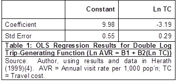
Herath follows the common practice of scaling up the survey data to reflect total annual visits, and then calculating the regression with annual visit rate per 1,000 population as the dependent variable. Personally, I prefer to scale up only after calculating a regression with an unscaled dependent variable (surveyed visits per capita). Either approach should yield the same results, but the latter is conceptually simpler when considering (as we will below) the variance of the dependent variable.

The analysis that follows will consider the precision of these coefficient estimates as measured by their standard errors. To focus on the key points at issue, I shall assume that all data were accurately measured and the trip-generating function was correctly specified as stated in Table 1, and ignore possible challenges to those assumptions.

In outline, there are two problems with the way in which these standard errors have been obtained. Firstly, standard errors estimated in the conventional way from the sum of squared residuals are subject to considerable sampling error when the sample size and therefore the number of residuals used in the calculation is small. The data points may just happen to be closer to or further from the fitted line than is representative of the population of possible zones around the site. Secondly, standard errors estimated by OLS are unreliable in the presence of heteroscedasticity, to which ZTCM is prone. The variance of a zonal visit rate will depend on the zonal population (larger population implies smaller variance) and on the visit rate itself (higher visit rate implies larger variance) (5).

What’s more, these two problems are difficult to separate since the small sample size also undermines some of the methods most commonly used in addressing heteroscedasticity. Inferences about the presence or form of heteroscedasticity from inspection or analysis of residuals are unreliable when the number of residuals is small. Use of robust (heteroscedasticity-consistent) standard errors is unreliable with small samples (6). Two-stage estimation, in which OLS estimates are used in obtaining weights designed to correct for heteroscedasticity in a second stage weighted least squares (WLS) estimation, is also unreliable because weights obtained in this way will be subject to considerable sampling error.

Let’s look more closely at how sampling error can affect the standard errors. The true variances (squares of standard errors) of estimates of regression coefficients are given by (7):

$Var[\hat{B}]= \sigma_0^2.(X'X)^{-1}\qquad(E1)$

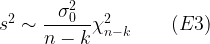
Here B is the vector of coefficients and X the matrix of values of the independent variables. $\sigma_0^2$ is the regression variance (the conditional variance of the error term). Since this is usually unknown it is standard practice to substitute for it the variance estimator $s^2$ , defined as below where SSR is the sum of squared residuals, n the number of observations, and k the number of coefficients estimated.

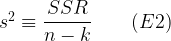
$s^2 \equiv \dfrac{SSR}{n-k}\qquad(E2)$

The problem with this is that the variance estimator, as its name suggests, is merely an estimator. It is an unbiased estimator of $\sigma_0^2$ , but unbiasedness is a repeated sample property, so the value of $s^2$ calculated from a particular sample may be either less or more than $\sigma_0^2$ . Considered over repeated samples, $s^2$ is a random variable with an approximately chi-square distribution given by (8):

$s^2 \sim \dfrac{\sigma_0^2}{n-k} \chi^2_{n-k}\qquad(E3)$

In the present case n = 5 and k = 2, so this reduces to:

$s^2 \sim \dfrac{\sigma_0^2}{3} \chi^2_3\qquad(E4)$

Although $\sigma_0^2$ is unknown, we can infer that the distribution of $s^2$ is proportional to that of a chi-square variable with 3 degrees of freedom. The distribution of such a variable is highly right-skewed. Although its mean is 3, its median is about 2.37, and the probability that its value is less than 3 is therefore well over half. In other words, it is not only possible but likely that $s^2$ will underestimate $\sigma_0^2$ and therefore that conventional standard errors will be underestimated. The distribution is also highly dispersed: its 25% and 75% percentiles are 1.21 and 4.11 respectively, and the 95% confidence interval is enormous, from 0.22 to 9.35.

So what can we do? It’s all very well to make the general observation that conventional standard errors calculated from very small samples and in the presence of heteroscedasticity are extremely unreliable. But can we determine whether the standard errors calculated from a particular dataset are too large or too small? There are two features of the present case that can help. One is the logged dependent variable which, as it happens, deals neatly with heteroscedasticity due to differing zonal populations. For a given zone, let V be the number of visits identified by the survey from that zone, N the zonal population, and VR the unscaled visit rate. Since N is a constant for any one zone so that Ln N is also a constant and Var[Ln N] is zero, we have:

$Var[Ln VR] = Var[Ln(V/N)] = Var[Ln V - Ln N] = Var[Ln V]+Var[Ln N]$

and so:

$Var[Ln VR] = Var[Ln V]\qquad(E5)$

Thus we have shown that Var[Ln VR] does not depend on N.

The other helpful feature is that the aggregate nature of the dependent variable enables us, on reasonable assumptions, to draw a conclusion about its variance. We start from the observation that the value of V, the number of visits from a particular zone identified by a survey, is a consequence of many separate decisions by the many individuals in that zone. Since it is unlikely that any individual will visit more than once within the scope of the survey, we can treat the number of visits v by an individual within the scope of the survey as a Bernoulli variable (equalling either 0 or 1). Writing p for the probability that v = 1, and using standard properties of the Bernoulli distribution, we have:

$E[v] = p\qquad(E6)$

$Var[v] = p-p^2\qquad(E7)$

We must expect that p varies between individuals within the zone: some will like visiting lakes more, or have more leisure time, than others. However, it is reasonable to assume that the p are all small, since people like variety in their leisure activity, so that even if someone likes visiting lakes and likes visiting that lake in particular, the probability that they will visit it within a particular period of a few days will be small. Hence the squared term in E7 can be ignored. It is also reasonable to assume that the p are largely independent, because decisions by one individual are unlikely to influence more than a tiny proportion (family members and a few friends, perhaps) of the thousands within the same zone). It can reasonably be assumed therefore that the distribution of V, the sum of the v for all the individuals in the zone, approximates to a Poisson distribution (9) with the properties:

$E[V] = Var[V] = \sum p\qquad(E8)$

where the sum is over all the individuals in the zone.

To use E8 to draw a conclusion about Var[Ln VR] we need to express the latter as a function of Var[V]. If Z is a Poisson variable with mean and variance $\lambda$ , a good approximation (obtained using a Taylor series expansion of the log function) is:

$Var[Ln Z] \approx \dfrac{12\lambda^2 + 18\lambda + 11}{12\lambda^3}\qquad(E9)$

Its error is between 3% and 6% for $\lambda$ between 5 and 10, falling to less than 1% for $\lambda$ greater than 20. Putting Z = V in E9 and substituting into E5, we have:

$Var[Ln VR] \approx \dfrac{12(E[V])^2+18E[V]+11}{12(E[V])^3}\qquad(E10)$

For convenience I will abbreviate the right-hand expression in E10 as g(E[V]). From E10 we can infer that heteroscedasticity due to differences in visit rates is still present after the log transformation. This can in principle be addressed by WLS estimation, the necessary weighting factor being the reciprocal of g(E[V]). This is equivalent to OLS estimation of the model (with u as the error term):

$(g(E[V]))^{-0.5}Ln VR)=(g(E[V])) ^{-0.5}B1+(g(E[V])) ^{-0.5}B2(Ln TC)+u\qquad(E11)$

To confirm that this is homoscedastic, we first show that the dependent variable is homoscedastic. Noting that g(E[V]) is constant for any particular zone and using E10 we have:

$Var[(g(E[V]))^{-0.5}Ln VR] = g(E[V])^{-1}Var[Ln VR] \approx g(E[V])^{-1}g(E[V])$

and so

$Var[(g(E[V]))^{-0.5}Ln VR] \approx 1\qquad(E12)$

Given our assumption that the regression model is correctly specified, we can infer that it is homoscedastic since for any zone the regression variance $\sigma_0^2$ is given by:

$\sigma_0^2 = Var[u] = Var[(g(E[V]))^{-0.5}Ln VR] \approx 1 \qquad(E13)$

However, the problem remains that we do not have reliable estimates of E[V] for each zone to slot into E11. We cannot therefore undertake a single definitive WLS estimation leading to coefficient estimates with reasonably reliable standard errors.

To make further progress, we can consider two cases. The pair of true values of the regression coefficients are either within or outside the 95% confidence ellipse defined by the OLS results. This ellipse (see Figure 1 below) is defined by the results in Table 1 together with the estimated covariance between the constant and travel cost coefficients. Its meaning is that, on repeated sampling and if the standard errors (and covariances) are correct, 95% of such ellipses will contain the true pair of coefficients. Note that Figure 1 is based on the unscaled visit rate (hence the range of the constant coefficient is much lower than its estimate in Table 1).

If the true coefficient values are outside this ellipse, it could be that the standard errors are correct and the sample data happens to be such that the ellipse is one of the unlucky 5%. This is an unlikely but not impossible scenario. Since we know that the standard errors are very unreliable, however, a more plausible interpretation is that the standard errors are too small, and that a confidence ellipse based on the true standard errors would have included the true coefficient values.

The case of true coefficient values within the ellipse requires a different type of reasoning. We select a representative sample of pairs of coefficient values from different regions of the ellipse. Since the ellipse is long and narrow, from top left to bottom right, I shall illustrate the method using three pairs of coefficient values identified as ‘top left’, ‘centre’ and’ bottom right’. For each such pair, we use the regression model to calculate the implied values of E[V] for each zone, and substitute these into E12 to obtain weights for WLS estimation of the model.

Having obtained the estimated coefficients and standard errors for each pair, there is a further important step to be taken. Given our conclusion (E13) that $\sigma_0^2$ approximates to 1, we can use that fact in calculating the standard errors, and need not rely on $s^2$ . If we have already obtained standard errors using $s^2$ , we can infer a convenient method of adjustment from the relation:

$Var[\hat{B}] = \sigma_0^2.(X'X)^{-1} = \dfrac{\sigma_0^2}{s^2}.(s^2.(X'X)^{-1}) \approx\dfrac{1}{s^2}.(Var[\hat {B}]_{Conv})\qquad(E14)$

Here the subscript ‘Conv’ identifies conventional estimates calculated using $s^2$ . From E14 we can infer this simple formula relating true standard errors (in this context) to conventional ones:

$se[\widehat{B_j}] \approx \dfrac{se[\widehat {B_j}]_{Conv}}{s}\qquad(E15)$

Table 2 below shows the results of the WLS estimations. All three estimations use the same underlying data; they differ only in the coefficient values used in obtaining the weights.

Table 2 shows that the standard errors obtained by WLS estimation and adjusted as described above are considerably higher than those in Table 1. The standard errors based on the top left point are 35% and 41% higher respectively for the constant and travel cost coefficients; for the other two points, the percentages are much higher. While it has not been proved that standard errors based on other points within the ellipse will also be considerably higher than those in Table 1, it appears a reasonable inference.

Whether the true values of the coefficients lie outside or inside the ellipse, therefore, we can conclude, to at least a reasonable degree of likelihood, that the standard errors in Table 1 are underestimated.

If we can dispense with $s^2$ in this way for this case, it might be asked, could the method be more widely used in econometrics? There are two reasons why its applicability is limited. Firstly, the reasoning that $\sigma_0^2$ approximates to 1 depends on the fact that we are dealing with data resulting from the aggregation of many independent binary decisions. Secondly, the fact that the sample size is so small means that any elements of approximation in that reasoning are relatively small in comparison with the imprecision of $s^2$ . That there are elements of approximation is not denied: an individual could visit more than once; individual decisions will not all be independent; the $p^2$ terms will not be exactly zero. A judgment has to be made, and mine is that, in the circumstances of this case, the reasoning that $\sigma_0^2$ approximates to 1 is much more reliable than the variance estimator. But if the sample were only a few times larger, say n = 20, the sampling error in $s^2$ would be much less and the judgment less clear.

Supporting Analysis

I can provide the supporting analysis on request (in MS Office 2010 format). My email address is in About.

Notes and References

1a. Rosenthal D H & Anderson J C (1984) Travel Cost Models, Heteroskedasticity, and Sampling Western Journal of Agricultural Economics 9(1) p 58-60; http://ageconsearch.umn.edu/bitstream/32368/1/09010058.pdf

1b. Hellerstein D (1995) Welfare Estimation Using Aggregate and Individual-Observation Models: A Comparison Using Monte Carlo Techniques American Journal of Agricultural Economics 77 (August 1995) p 623

2. Herath G (1999) Estimation of Community Values of Lakes: A Study of Lake Mokoan in Victoria, Australia Economic Analysis & Policy Vol 29 No 1 pp 31-44

3. Herath, as 2 above, p 35.

4. Herath, as 2 above, p 37.

5. Christensen J & Price C (1982) A Note on the Use of Travel Cost Models with Unequal Zonal Populations: Comment Land Economics 58(3) pp 396 & 399

6. Imbens G W & Kolesar M (Draft 2015) Robust Standard Errors in Small Samples: Some Practical Advice pp 1-2 https://www.princeton.edu/~mkolesar/papers/small-robust.pdf

7. Ruud P A (2000) An Introduction to Classical Econometric Theory Oxford University Press p 157. Note that the argument of E1 to E4 assumes both homoscedasticity and normality of error terms (but it would be optimistic to expect that conventional standard errors would be more reliable when these assumptions do not hold).

8. Ruud, as 7 above, p 199

9. The distribution of V approximates to a Poisson binomial distribution, and this in turn approximates to a Poisson distribution. See Hodges J L Jr & Le Cam L (1960) The Poisson Approximation to the Poisson Binomial Distribution The Annals of Mathematical Statistics 31(3) pp 737-740 http://projecteuclid.org/euclid.aoms/1177705799

Posted in Recreation | Tagged heteroscedasticity, small sample size, zonal travel cost method | Leave a comment

Zone Definition and Travel Cost Valuations

Posted on June 21, 2016 by Adam Bailey

The literature on the zonal travel cost method (ZTCM) contains occasional suggestions that results can be sensitive to zone definition. My exploratory analysis strongly supports this view.

Originally posted 14/5/2014 as “The Travel Cost Method – Another Pitfall”. Re-posted following site reorganisation 21/6/2016.

In a previous post, I outlined some well-known pitfalls of the travel cost method. Here I describe and illustrate a pitfall of the zonal version of the method that seems not to be as well-known as it should be.

Introduction

It is generally accepted that research results should be replicable. For a zonal travel cost study, replicability most obviously requires that the same method of analysis applied to data from repeated on-site surveys should lead to similar results. Another requirement, I propose, is that repeated analysis of data from a single on-site survey, aggregated within different zone specifications, should also lead to similar results. I shall refer to this as zonal replicability.

What is the basis for this second requirement? One argument refers to the general scientific maxim, discussed in this post, that repeated tests or measurements should replicate the essential and vary the inessential. Organising points of visitor origin into zones is an essential feature of the zonal travel cost method, but the particular zone specification (often driven by data availability) can hardly be regarded as essential. A more specific argument focusses on the central assumption of the travel cost method, namely, that people would respond to a site entrance fee in the same way that they are found to respond to an equivalent travel cost. This assumption, though it can be challenged, has at least some intuitive plausibility. Suppose however that we were to identify a particular zone specification, and make the assumption that people would respond to a site entrance fee in the same way that they are estimated, using that zone specification, to respond to an equivalent travel cost. An assumption which privileged one particular zone specification in this way would lack plausibility, since it would beg the question whether alternative zone specifications would lead to different findings.

There are many references in the ZTCM literature to the problem of aggregation bias, that is, trip-generating function parameters estimated from aggregate data generally may not accurately reflect individual behaviour (1a-b). It is, perhaps, a short step to the idea that different aggregation structures might yield results that are biased to different degrees or in different directions, but rarely has this step been taken. A notable exception is Bateman (1993), who identified as a feature of ZTCM the possibility of increasing or reducing valuation estimates by respecifying zones (2).

A ZTCM study by Gillespie Economics (2007) includes a statement that consumer surplus estimates were tested for sensitivity to zone specification (3). However, little detail was provided as to the number of alternative zone specifications and how they were chosen. It is unclear therefore how much weight can be placed on the reported finding that differences in consumer surplus estimates were less than 2.5%.

Early applications of ZTCM specified zones consisting of concentric rings. Sutherland (1982) demonstrated that consumer surplus estimates could be sensitive to ring width (4). However, most recent applications of ZTCM use irregular zone specifications, often based on administrative or census districts. My analysis considers the effect on results of alternative irregular zone specifications.

Method

A special case of zonal replicability relates to alternative zone specifications obtained by selective merging of a study’s original zones. If results are found not to be replicable even in such a case, then a fortiori they will not be replicable across the full range of alternative zone specifications. I explored replicability of this kind using data from a study by Rathnayake and Gunawardena (2011) of Horton Plains National Park, Sri Lanka (5), which I chose mainly because unlike many published studies it discloses its full zonal data. This study used data on a sample of visitors, aggregated within 17 of Sri Lanka’s districts together occupying most of the centre and south of the island. Map 1 below shows the 17 district zones, and Chart 1 plots the original zonal data.

My re-analysis of the data followed the original study in treating travel cost as the only independent variable in the trip-generating functions and assuming a linear functional form. However, to address heteroscedasticity I departed from the original study in estimating the trip-generating functions using weighted least squares, giving higher weightings to zones with larger populations and/or lower visit rates, characteristics which theory suggests will be associated with lower variability in visit rates (7a-b).

To explore zonal replicability, I first obtained a random sample of alternative zone specifications. The purposes of the sample were: firstly, to support inferences about a wider population of alternative zone specifications without having to make separate calculations for each specification; and secondly, to facilitate illustration of the range of results from alternative zone specifications with examples that cannot plausibly be dismissed as highly unusual or ad hoc constructions.

The sample frame consisted of all possible groupings of the 17 districts into eight zones consisting of seven pairs and one triple, the districts within each pair and triple being required to be adjacent (8). The number of such groupings was found to be 356. A sample of 30 zone specifications was then selected by simple random sampling. Visit rates and travel costs for each merged zone were calculated as population-weighted averages of their values for its constituent districts. The trip-generating functions for each of the 30 zone specifications were then estimated, and from these the demand curves and consumer surpluses were obtained in the standard way (9).

From the distributions of the estimates of the trip-generating function coefficients and consumer surplus over the sample of 30 zone specifications, inferences were drawn about their distributions over the population of 356 zone specifications.

Results

A convenient unit-free measure of the variability of a distribution is its coefficient of variation, the ratio of its standard deviation to its mean. Table 1 shows the estimated coefficients of variation of the distributions of the trip-generating function coefficients over the population of 356 zone specifications. The variability measured here is due solely to different zone specifications applied to the same underlying data. It is quite distinct from the imprecision of individual coefficient estimates arising from the underlying data being sample-based.

The two coefficients are negatively correlated, a higher constant being associated with a more negative travel cost coefficient, and the estimated trip-generating functions intersect in the region where most of the original data points are concentrated. Chart 2 shows the trip-generating functions with the highest and lowest constants among the sample, illustrating the range of variability and the intersection property, and Maps 2 and 3 show the relevant zone specifications.

Chart 3 shows the distribution of consumer surplus estimates within the sample. The coefficient of variation is 0.222, larger than for either of the trip-generating coefficients. The highly skewed distribution suggests that the distribution of consumer surplus estimates over the population of 356 zone specifications may be far from normal, and there was therefore no simple way to estimate the coefficient of variation of that distribution. Nevertheless, the range of estimates over the population must be at least as large as that over the sample, which is from R’s 36.4 M (Specification 13) to R’s 76.7 M (Specification 26), a factor of 2.1.

Discussion

The finding that different zone specifications can lead to different results is an example of a general problem in spatial modelling, known to geographers and statisticians as the modifiable areal unit problem. In general terms, the problem is that spatial data can be aggregated in many different ways which can lead to different results on analysis of the aggregate data. A useful source is Openshaw (10). A rare reference to the problem in the literature on the travel cost method is by Brainard, Lovett & Bateman 1997, who characterise that literature, with some justice, as spatially naïve (11).

The finding that the variability over different zone specifications of the consumer surplus estimates can be greater than that of the trip-generating function coefficients parallels a similar finding by Adamowicz, Fletcher & Graham-Tomasi (1989) in respect of variability arising from sampling error (12). An underlying reason in both cases is that, even if the trip-generating function is linear, there is non-linearity in the calculation of the consumer surplus from the trip-generating function.

It was not an aim of this analysis to test the replicability of the results of the original study by Rathnayake & Gunawardena. A comparison of the results from alternative specifications of 8 zones with those from the original specification of 17 zones would conflate two issues: the effect of alternative specifications of a given number of zones, and the effect of varying the number and size of zones. That specifications with more and smaller zones will tend to exhibit less variability in their results than those with fewer and larger zones is an interesting and plausible hypothesis, but not one that has been explored here. The most direct relevance of this analysis is to ZTCM studies where the original zone specification consists of about 8 zones.

Examples of such zone specifications that have been used in ZTCM studies include South African provinces (9 zones), Ugandan districts (10 zones), groups of Indian states (10 zones), groups of Chinese provinces (9 zones), and (for a site attracting many international visitors) a specification based largely on continents (7 zones) (13a-e). Given the finding that alternative specifications of 8 zones around the Sri Lankan site can lead to results differing by a factor of more than 2, it seems likely that results based on specifications of 7-10 zones in other parts of the world would be found to vary markedly with the particular specification chosen, holding the number of zones constant. If so, results based on one particular specification are fairly likely to be markedly biased (since if different specifications lead to a wide range of results, only a small proportion can lead to results that approximate closely to the true result). Moreover, if the result of a ZTCM study based on about 8 zones is presented simply as a point estimate of consumer surplus, then it is likely to lack zonal replicability.

Should it be inferred that ZTCM is so unreliable that it should be abandoned? That would be too sweeping a conclusion I suggest. All methods for valuing non-market environmental goods have their limitations, and we need ZTCM among our menu of available methods, especially for circumstances in which aggregate data is all we can collect at reasonable cost. What certainly should be inferred is that the results of ZTCM studies should be presented in a way which clearly communicates their possible inaccuracy. This requires explicit reference both to sampling error arising from the underlying data being sample-based and possible bias arising from the choice of zone specification to aggregate that data. A useful topic for further research would be to test the hypothesis that variability in results can be reduced by specifying smaller zones, with a view to developing guidance on zone size.

Supporting Analysis

I can provide the supporting analysis on request (in MS Excel 2010 format). My email address is in About.

Notes & References

2. Bateman I J (1993) Valuation of the environment, methods and techniques: revealed preference methods, in Turner R K (ed) Sustainable Environmental Economics and Management: Principles and Practice Belhaven Press, London p 230

3. Gillespie Economics (2007) The Recreation Use Value of NSW Marine Parks (Report for the New South Wales Department of Environment and Climate Change) p 4 http://www.environment.nsw.gov.au/resources/research/RecreationUseValueNSWMarineParks.pdf

4. Sutherland R J (1982) The Sensitivity of Travel Cost Estimates of Recreation Demand to the Functional Form and Definition of Origin Zones Western Journal of Agricultural Economics July 1982 pp 95-7 http://ageconsearch.umn.edu/bitstream/32416/1/07010087.pdf

5. Rathnayake R M W & Gunawardena U A D P (2011) Estimation of Recreational Value of Horton Plains National Park in Sri Lanka: A Decision Making Strategy for Natural Resources Management Journal of Tropical Forestry and Environment 1(1) pp 71-86 http://journals.sjp.ac.lk/index.php/JTFE/article/view/86

Rathnayake & Gunawardena, as 5 above, pp 79-80

7a. Bowes M D & Loomis J B (1980) A Note on the Use of Travel Cost Models with Unequal Zonal Populations Land Economics 56(4) p 468

7b. Christensen J B & Price C (1982) A Note on the Use of Travel Cost Models with Unequal Zonal Populations: Comment Land Economics 58(3) pp 396 & 399

8. Identifying all such groupings was a challenging mathematical problem, solved by a method involving representation of each district by a distinct prime integer, and each pair and triple by the product of the primes representing its constituent districts. The use of products of distinct primes ensures that zones are non-overlapping if and only if their products have no common factor greater than one. In this way the spatial problem was transformed into an arithmetical problem which could be solved in a spreadsheet.

9. See for example Perman R, Ma Y, McGilvray J & Common M (3^rd ed’n 2003) Natural Resource & Environmental Economics Pearson / Addison Wesley, Harlow, England pp 413-4

10. Openshaw S (1984) The Modifiable Areal Unit Problem Geo Books, Norwich, England http://qmrg.org.uk/files/2008/11/38-maup-openshaw.pdf

11. Brainard J S, Lovett A A & Bateman I J (1997) Using isochrone surfaces in travel-cost models Journal of Transport Geography 5(2)p 118

12. Adamowicz W L, Fletcher J J & Graham-Tomasi T (1989) Functional Form and the Statistical Properties of Welfare Measures American Journal of Agricultural Economics 71 pp 416 & 418

13a. Turpie J & Joubert A (2004) The value of flower tourism on the Bokkeveld Plateau – a botanical hotspot Development Southern Africa 21(4) pp 647 & 650

13b. Buyinza M, Bukenya M & Nabalegwa M (2007) Economic Valuation of Bujagali Falls Recreational Park, Uganda Journal of Park and Recreation Administration 25(2) p 21 http://js.sagamorepub.com/jpra/article/view/1362

13c. De U K & Devi A (2011) Valuing Recreational and Conservation Benefits of a Natural Tourist Site: Case of Cherrapunjee Journal of Quantitative Economics 9(2) p 162

13d. Liu Y, Nie L & Liao B (2012) The Recreational Value of Bama in China: One of the Five World’s Longevity Townships Business and Management Research 1(4) p 149 http://www.sciedu.ca/journal/index.php/bmr/article/view/2104

13e. Mugambi M D & Mburu J I (2013) Estimation of the Tourism Benefits of Kakamega Forest, Kenya: A Travel Cost Approach Environment and Natural Resources Research 3(1) p 65 http://www.ccsenet.org/journal/index.php/enrr/article/view/20073

Posted in Recreation | Tagged modifiable areal unit problem, zonal replicability, zonal travel cost method, zone specification | Leave a comment

Economic Droplets

Fishing and Economic Welfare