If we can value ecosystem services, then the “housing v countryside” debate can be treated as an optimisation problem.

Cities often expand laterally to provide housing for an increasing population. This usually involves a loss of surrounding farmland, woodland, wetlands or other countryside, and consequent loss of the ecosystem services they used to provide.  Opinions on housing and the countryside often tend towards one of two extreme positions.  There is the view that land must always be made available to meet some conception of “housing need”, regardless of the resulting destruction of the countryside.  At the other extreme is the view that countryside around cities (Green Belt as some is designated in the UK) should be inviolable, implying that “urban sprawl” should always be prevented.

An Economic Model of Land Use In and Around a City

Economic analysis offers a way to articulate a third view.  To anyone with a little economic training the following formulation may seem quite natural, a straightforward application of the equimarginal principle of optimisation to the case of different land uses:

Overall welfare is maximised if housing extends up to, but not beyond, the point at which the marginal value of housing per unit of land equals the marginal value of an undeveloped unit of land.

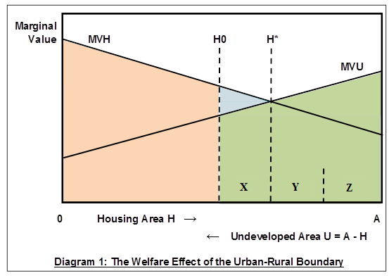
This is represented in Diagram 1 below.  Line MVH shows the marginal value of housing, falling as housing area is increased. Line MVU shows the marginal value of undeveloped land, rising as housing area is increased and therefore less undeveloped land remains.  In the case shown, the area occupied by housing is H0, the red area represents the total economic value of housing, and the green area the total economic value of undeveloped land within the relevant area.  However, overall welfare is maximised where the respective marginal values are equal, that is, at the intersection of the marginal value lines, with housing area H*, and declines with distance from H* on either side.  With housing occupying area H0, therefore, welfare is less than it might have been by the amount represented by the blue triangle (though more than it would have been if H0 had been even further to the left of H*).

Now I do indeed think that this is a useful model to have in mind when considering policy towards housing development. Nevertheless, the assumptions on which it relies are considerable.  Awareness of those assumptions can help to ensure that we do not misapply the model.

I begin with some general remarks about assumptions in relation to economic models.  Some assumptions are just convenient simplifications, useful for presenting a model but readily replaced by more realistic descriptions in empirical work that pretends to any degree of accuracy.  Others are more essential to the model, indicating limitations in scope beyond which it would not work or be fundamentally altered. In the present case, the assumption of  linearity of the marginal value lines is just a convenient simplification.  The fact that these lines are monotonic (downward sloping in one case and upward sloping in the other) is more essential: if instead the lines were complex curves with both downward and upward sloping regions, then there could be multiple local optima at which the marginal values were equal, and welfare would not always be lower if H0 were further from the global optimum.

The spatial and temporal frameworks of the model require comment.  The assumption that all relevant land is either undeveloped or used for housing ignores other urban land uses (businesses, roads and railways, urban parks, etc) but is a convenient simplification.  The same can be said of the assumption that there exists a fixed area of “relevant land” in and around a city. What matters for the model is that it considers the respective marginal values over the range of areas of land relevant to a particular question. In terms of the diagram, moving A a little to the left or right will not change either the position of H* or the area of the blue triangle.  Similarly, it could be acceptable to truncate the diagram at the left, setting the origin at, say, 500 hectares rather than at zero area. This would change the position of H* only in the trivial sense that it would be closer to the new origin.  Its true position relative to the area indicated by the horizontal scale would be unaffected.

A measure of welfare should relate to a defined period.  It is convenient to take the period to be short (one year at most), since then in most circumstances we can ignore additions to the housing stock during the period.  This is a reasonable assumption because additions to housing in any period are usually only a very small proportion of total stock. Policy on housing development relates to the model in that the housing stock reflects policies in many past periods, which may or may not have changed the quantity or character of housing development from that which would have been delivered in a free market.  Thus the model relates welfare in a period to the outcome of policy and market forces in many previous periods.  What the model does not do, and it is a significant limitation, is draw out the full consequences of policy at any time for welfare extending over many periods.

Nor is the model designed to show the welfare effects of possible additional housing development.  That would require consideration of housing construction costs, which do not feature in the model (the assumption of no additions implies that all construction costs were incurred in past periods and are therefore sunk costs, irrelevant to welfare in the period of interest).  Any welfare comparisons inferred from the model are not comparisons before and after new development.  They are comparisons involving one or two hypothetical alternatives to the actual situation in the period, based on counterfactual assumptions about the quantities of housing development in past periods.

The Value of Land with Housing

Consider now the marginal value of housing line.  Because the horizontal axis measures land area, the line must be taken to mean the marginal value of housing per unit of land area.  A simple interpretation of the line starts from assumptions of uniform housing density and uniform utility to residents per home.  Given these assumptions, residents have no reason to prefer one home to another.  Ignoring externalities (which we will consider below), the marginal value of housing line would therefore be a pure price-quantity relation, its downward slope reflecting the greater quantity demanded of housing of uniform utility when the price of housing is lower.

Suppose that, with a view to greater realism, we drop the uniform utility assumption and take it instead that, although housing is of uniform density, homes differ in attributes such as quality and location which determine their utility to residents.  Then we must expect the price of housing in a particular location per unit of land to depend upon both its attributes and the total quantity of housing.  But if homes are not equivalent, on which land shall we take the marginal unit of housing to be?  For the purposes of economic welfare analysis, we should ignore geographical considerations, such as distance from the city centre, and take units of land in descending order of utility of their housing.  Thus the marginal unit of land with housing is that at which the homes offer the least utility.

Table 1 below shows how this would work for a very simple case with just three land units, identified in descending order of utility as L1, L2 and L3.  H is the number of units occupied by housing and, given uniform housing density, also measures the quantity of housing.  The locations have demand functions with the same downward slopes with respect to housing quantity, but different choke prices reflecting their different utility.  In the demand columns, an entry of “na” against an area indicates that it would have no housing at the relevant value of H.

The entries in red trace the marginal value of housing line: if for example H = 2, then the marginal unit is L2 for which demand is 11.  Note that, unlike in the case of uniform utility, this line is not a pure price-quantity relation.  Of the fall in marginal value of 7 from H = 2 to H = 3, for example, 2 is due to the higher quantity of housing and 5 to the lesser utility of L3 than L2.

Thus we can derive a downward-sloping marginal value of housing line without assuming uniform utility, at least within the area of existing housing.  To extend the line into the area of undeveloped land, we would need to make an assumption about the quality of the homes that might be built on that land.

Even within the area of existing housing there are further issues with the concept of the marginal value of housing line.  We have noted that location is an attribute that can affect the utility offered by a home.  Some characteristics associated with location, such as risk of subsidence or flooding, may be permanent.  Within a city, however, most of the utility associated with a home location relates to ease of access to and quality of shops, schools, transport links, employment opportunities, business and social networks, parks, and so on.  Importantly in this context, differences in housing quantity at the margin can be associated with differences in the locational attributes of intra-marginal homes.  In other words there can be positive or negative externalities associated with particular homes, that is, social benefits or costs not accruing to or borne by residents of those homes.  Comparing situations with larger and smaller numbers of residents, the former may for example have more or better shops, different social mixes in schools, more congestion on roads and public transport, and more networking opportunities. Such externalities imply that the utility of any one home is not fixed but may depend upon the quantity and location of other homes.  Consequently, an ordering of land units defined in terms of housing utility may itself not be fixed.

In most cities the density of housing is far from uniform (with the inevitable consequence that there is no simple relation between housing area and quantity of housing (whether measured as number of homes or as floor space).  One way to handle this within the model is to treat density as another characteristic of location.  Thus demand for housing on a unit of land on which there is a tower block containing many flats will be the sum of the demands for the individual flats.  Subject to quality, that housing will have a much higher value per unit of land than land with low-rise homes, and so feature earlier in the ordering of land units.

Another approach starts from the observation that, in some cities, most high-rise housing developments are towards the centre.  For such cities, it may be a reasonably good approximation to reality to treat the outer suburbs as being of uniform density.  One might then exploit the possibility noted above of truncating the model at an area chosen so as to exclude most high-rise developments.

Unfortunately these approaches, though consistent with our model, are unsuited to addressing the important practical issue of selecting the appropriate density for new housing developments.  As many have pointed out, building housing at fairly high densities, either on undeveloped land or by redevelopment of urban sites, can limit the extent to which cities impinge on their surrounding countryside.  In this context, we really need a more complex model which considers how welfare can be maximised when both the area of land used for housing and the density of housing on that land are considered variable.  That is beyond the scope of this post.

A further issue concerning the marginal value of housing line is the definition of the underlying concepts of demand and price.  Since the model relates to a period, demand must be taken to mean demand for the use of housing for the period by both tenants and owner-occupiers, sometimes termed demand for housing services. Tenant demand can be equated with willingness to pay a period’s rent for a home.  Owner-occupier demand for a period’s use of housing is a theoretical construct that would have to be inferred from market data, with suitable adjustments to exclude the effect of any speculative element in market values.  That has its complications, but without such a concept of housing demand it is hard to see how economic welfare analysis can be applied to housing.

The Value of Undeveloped Land

The economic value of the undeveloped land is the total value of the various ecosystem services it provides over the period.  It includes the market value of the agricultural products of farmland less the costs of inputs other than land.  Often more important, however, are the values of non-market services including water purification, drainage, support for biodiversity, carbon sequestration, and opportunities for outdoor recreation. These values would have to be estimated using suitable non-market environmental valuation techniques (1). Some of these techniques are contentious, and none can be expected to yield more than very approximate value estimates.

If we assume that the ecosystem services are uniform across the land, then we can interpret the marginal value of undeveloped land line as a pure value-quantity relation.  Whether such a line would be upward-sloping would depend on the type of land use.  If the undeveloped land were all used for agriculture and were all of similar quality for that use, then its value might be roughly proportional to its area. Agricultural products from farmland may be sold on markets supplied by many regions, and the small changes in total market supply that would result from changes in the amount of farmland around one city would not significantly affect prices.  Proportionality would also probably apply to woodland if its main value elements were timber sold on markets supplied by many sources, and carbon sequestration contributing through atmospheric mixing to mitigation of the global increase in atmospheric greenhouse gases.  The model will work with a horizontal marginal value line for undeveloped land, provided that the marginal value of housing line slopes down so that the lines meet only at one point.

For some other land uses, the marginal value will be greater if there is less undeveloped land.  This applies especially to recreation.  If there is much open-access countryside within easy reach of a city’s inhabitants, then a little more or less would be unlikely to be of much consequence, but if only a little remains, then its marginal value would probably be considerable.  Recreational land much further from the city could not be considered an adequate substitute, given the greater travel costs city residents would have to incur to enjoy it (2).  It could also apply to aspects of biodiversity.  An animal species usually needs to forage or hunt for food, and this may be impossible if the remaining area of otherwise suitable habitat is too small, leading to loss of the species from the locality.   For such land uses, the marginal value of undeveloped line might be expected to slope upwards with increasing use of land for housing.

In most circumstances, however, the mix of ecosystem services provided by a unit of land will differ between units.  Provisioning services such as food crops and timber may relate to clearly delineated subsets of the total undeveloped area.  The rate of carbon sequestration is likely to be highest in areas of woodland, lower in areas with fewer trees, and close to zero in some other areas.  Support for biodiversity, which embraces many different plants and animals requiring different habitats, will vary according to the characteristics of different locations, and in some cases (eg where agricultural pests are present) could include negative value elements.  The effectiveness of water purification and drainage services will vary with geological and soil characteristics.

This leads to a problem analogous to that encountered above in respect of housing.  Where units of undeveloped land differ in ecosystem services and therefore in value, which piece of land should be taken to be the marginal unit?  Again, the economic approach is to take units of undeveloped land in descending order of value, reading in this case from right to left in our diagram.  As with housing land, the slope of the marginal line may then reflect a combination of differences in ecosystem services between land units and quantity effects.

Does the Model Identify the Welfare Optimum?

Let’s now bring together our analyses of the two marginal value lines.  Given the ordering approach to the construction of the two marginal curves, we can identify the marginal unit of undeveloped land and, in terms of the housing land ordering, the first extra-marginal unit of undeveloped land suitable for housing.  Suppose, to keep things simple, that the undeveloped land in Diagram 1 has been divided into just three units, X, Y and Z (and take the sloping marginal value lines as approximate representations of the step functions which such large units would require).  We might then identify X as being both the marginal unit of undeveloped land and the first extra-marginal unit of undeveloped land suitable for housing.  Since the marginal value of unit X as land for housing is greater than its marginal value as undeveloped land, we might infer (as suggested by the blue triangle) that welfare would be higher if X had been developed for housing.

But this is a fallacy.  Our orderings for housing and for undeveloped land are based on different principles. To make even partial sense of our diagram in circumstances of non-uniformity, we must specify that units of land with housing (to the left of H0) have been ordered according to value as housing, while units of undeveloped land (to the right of H0) have been ordered according to value as undeveloped land.  We cannot assume that the units of undeveloped land have the same ordering according to value as housing.  Table 2 below shows two (of several) possible ways in which the respective orderings of the undeveloped land might relate to each other.  Note that both possibilities have the same three values in the “Value as housing” column: only the orders differ.

Possibility 1 is the interpretation which Diagram 1 invites, with unit X having a higher value as housing.  But Possibility 2 is entirely plausible.  For example, unit Z might be attractive green space close to the edge of the city and have the highest value as undeveloped land because it receives many recreational visitors, but also because of its closeness to the city  have the highest value as housing.

Conclusion

The model clearly has many limitations.  I would justify the claim that it is nevertheless useful in the following ways.  Firstly, it offers a principled intermediate position on housing and the countryside as an alternative to the two extreme views outlined at the start of this post.  Even if it is challenging to estimate the marginal value lines for a particular city, the idea that welfare is maximised when the marginal values are equal is an important one whose recognition could raise the level of public debate on proposed housing development.  Secondly, the possibility of truncating the scope of the model – applying it to a relatively small area of land at the urban-rural fringe rather than to a whole city and a large area of surrounding countryside – could in some circumstances enable it to be applied in a relatively simple form because assumptions of uniformity would approximate to reality fairly well within that limited area.  Thirdly, it may be found that for some cities the difference in estimates of the marginal value of housing and undeveloped land is so large that – notwithstanding limitations of the model and the approximate nature of such estimates – a conclusion that welfare is far from being maximised would be hard to dispute.  That would not lead directly to a policy conclusion – whether or not to permit housing development on undeveloped land – but it would give a strong pointer suggesting a need for more detailed studies of particular sites near the urban-rural boundary.

Notes and References

1. For an overview of such methods see Joint Nature Conservation Committee – Ecosystem Services Valuation http://jncc.defra.gov.uk/default.aspx?page=6383.   I have discussed some of these methods in previous posts: see especially here re the travel cost method and here re contingent valuation.
2. Re the value of recreational land near to urban centres see Bateman I et al (2013) Bringing Ecosystem Services into Economic Decision-Making: Land Use in the United Kingdom Science Vol 341 Issue 6141 pp 45-50 (section headed National-Scale Implications)  http://science.sciencemag.org/content/341/6141/45